Visualise Data

A.H. Sparks

2024-05-04

library("tidyverse")
library("lubridate")
library("clifro")
library("viridis")
library("ggpubr")
library("here")
library("ChickpeaAscoDispersal")

theme_set(theme_pubclean(base_size = 14))

Visualise Counts per Pot

ggplot(lesion_counts, aes(x = m_lesions)) +
   geom_density() +
   xlab("Mean lesion count per plant")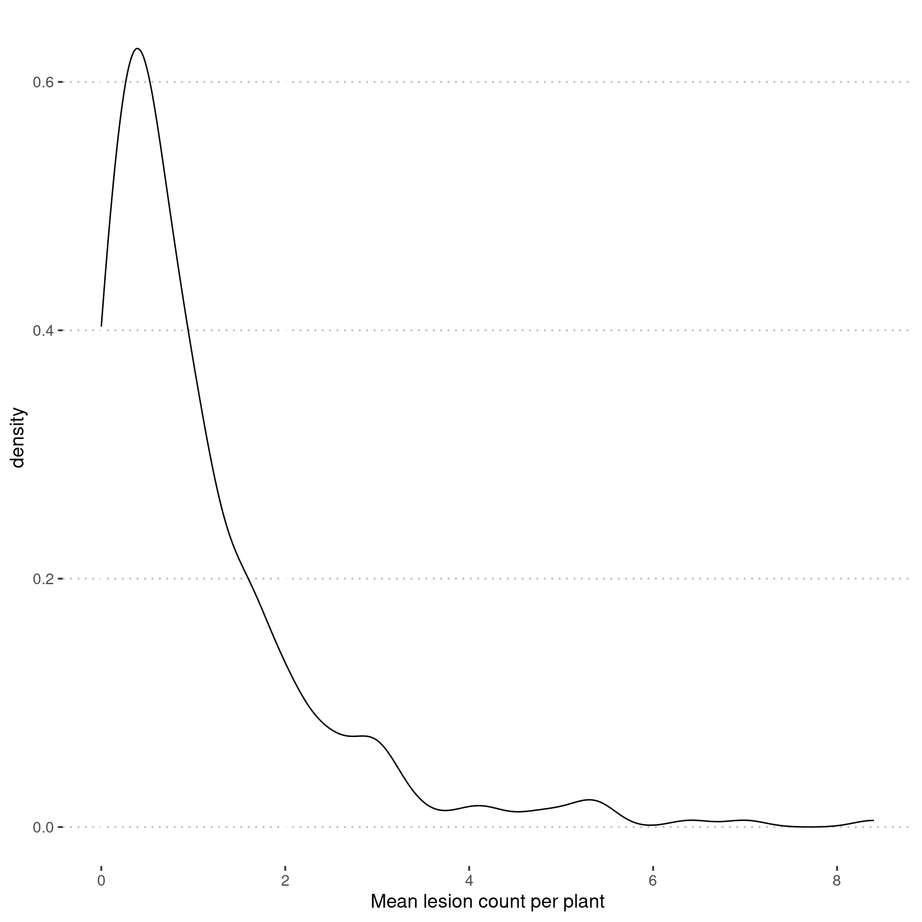

Density plot of mean lesions counted per plant for all six events.

Visualise the Dispersal Data

ggplot(lesion_counts, aes(x = distance,
                          y = m_lesions)) +
   geom_count() +
   scale_size(breaks = c(1, 2, 4, 8)) +
   stat_summary(fun.y = "median",
                geom = "line",
                na.rm = TRUE) +
   stat_summary(
      fun.y = "median",
      colour = "red",
      size = 2,
      geom = "point"
   ) +
   scale_x_continuous(breaks = c(0, 10, 25, 50, 75)) +
   ylim(c(-0.5, 9)) +
   ylab("Mean lesion count values") +
   xlab("Distance (m)") +
   facet_wrap(. ~ SpEv, ncol = 3)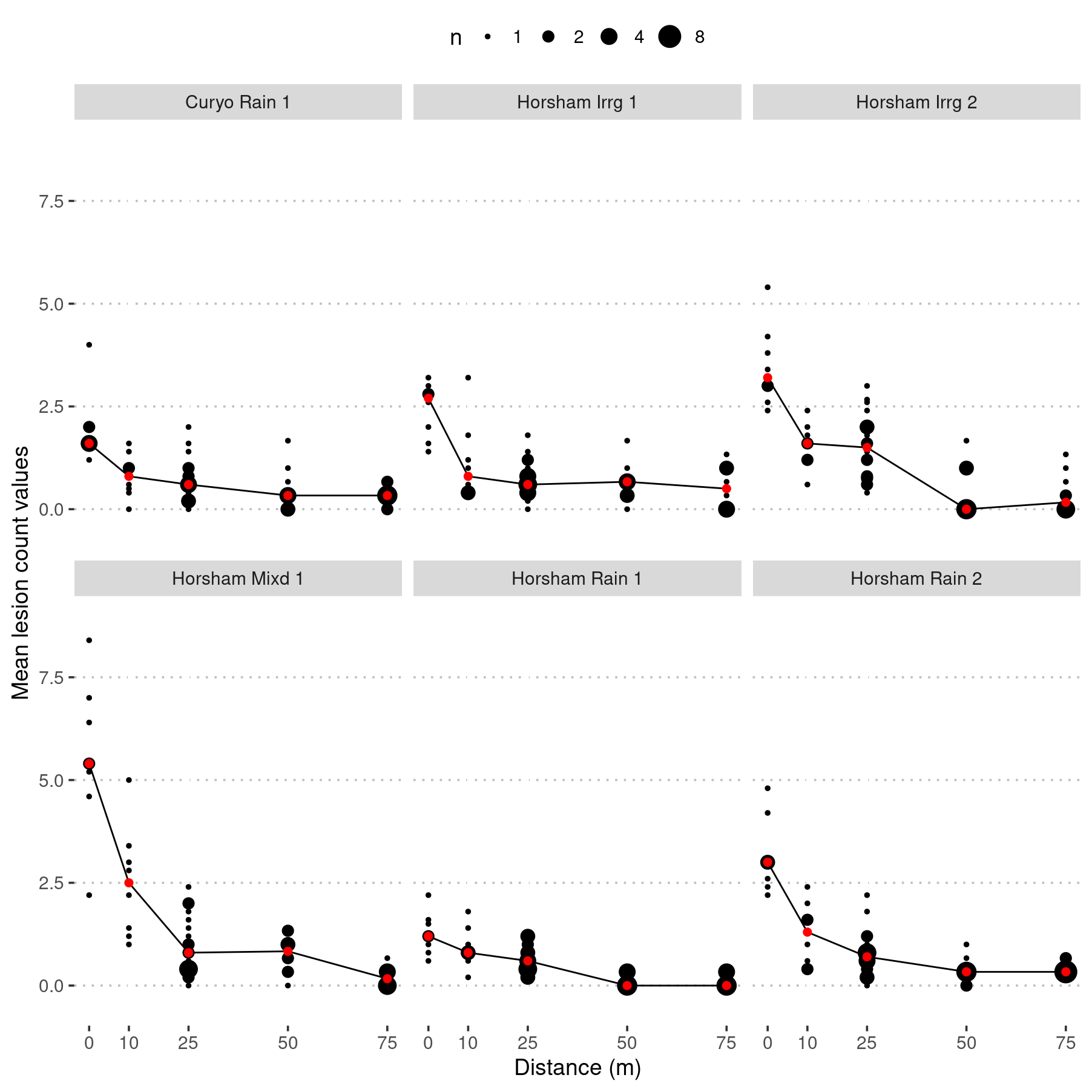

Mean number of conidia dispersed (counted as lesions) per plant during each spread event. Where the mean lesions per plant for each pot is shown on the y-axis and distance dispersed is on the x-axis. ‘n’ indicates the count of pots with the same mean lesions per trap plant, and is represented by point size. Red points and line show median lesions counted per trap plant. Conidia travelled up to 75 m in each of the six irrigation and rainfall event.

Visualise the Rainfall

dat <- left_join(lesion_counts, cleaned_weather, by = c("site", "rep"))

dat %>%
   group_by(SpEv) %>%
   mutate(Hour = floor_date(time, "1 hour")) %>%
   group_by(SpEv, Hour) %>%
   summarize(sum(rainfall)) %>%
   ggplot(aes(x = Hour, y = `sum(rainfall)`)) +
   geom_col() +
   scale_x_datetime(
      "Date (day-month)",
      date_breaks = "day",
      date_labels = "%d-%m",
      date_minor_breaks = "hour",
      guide = guide_axis(check.overlap = TRUE)
   ) +
   ylab("Precipitation (mm)") +
   facet_wrap(. ~ SpEv, ncol = 3, scales = "free_x")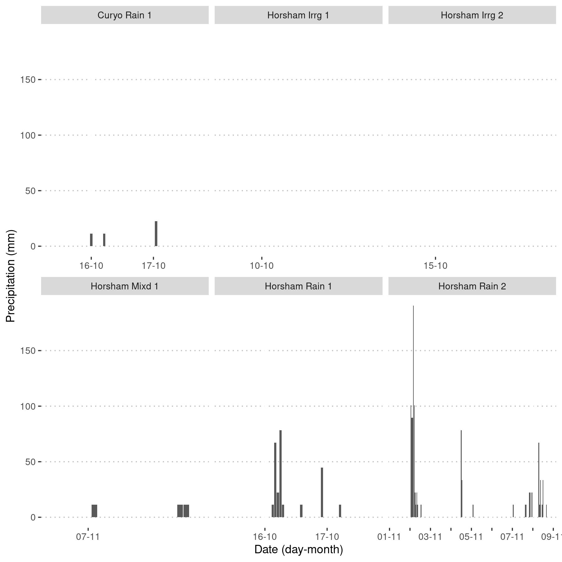

Ten-minute precipitation data for each of the six rainfall or irrigation events at two locations. Events are denoted by the location, ‘Horsham’ or ‘Curyo’; and whether the site was irrigated, ‘Irrg’ or rainfed ‘Rain’ or ‘Mixd’ (both simultaneously); and event ‘1’, ‘2’ or ‘3.’ Precipitation values, 11 mm that were applied, are not shown, only rainfall data are presented.

Visualise the Wind Speed and Direction

pw <-
   with(
      dat,
      windrose(
         wind_speed,
         wind_direction,
         SpEv,
         n_col = 3,
         legend_title = "Wind speed (m/s)"
      )
   )
pw +
   scale_fill_viridis_d(name = "Wind Speed (m/s)", direction = -1) +
   xlab("") +
   theme_pubclean()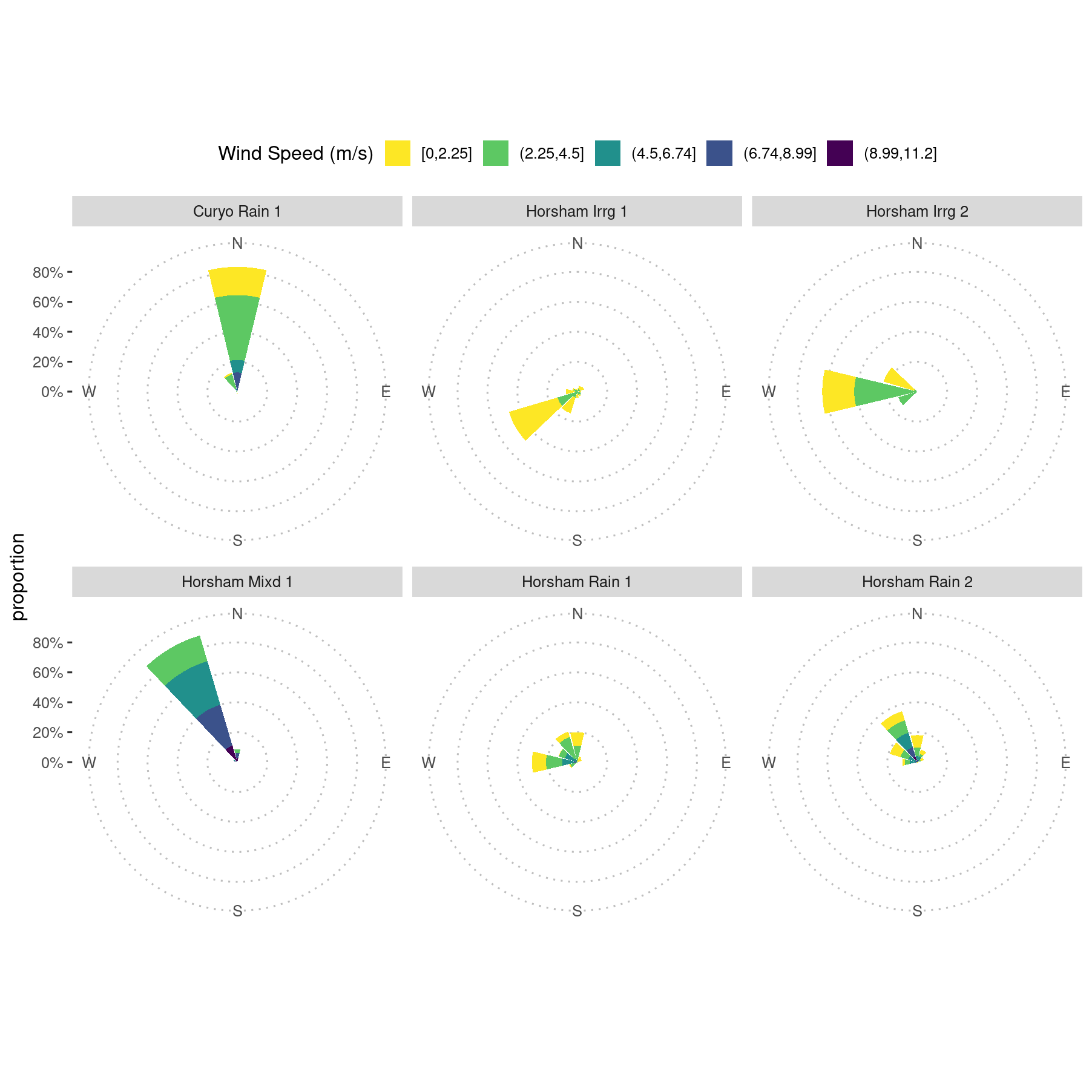

Windroses for spread events showing ten-minute wind speed and direction at the two Horsham sites. Curyo wind speed and direction data are not shown due to a weather station calibration issue resulting in incorrect data for wind direction.

When inspecting these data, we noted that the wind direction for Curyo was against the direction of spread along the transects, which led to further investigation of the weather data. That investigation is detailed in this analysis.

Heatmap of Lesions Along Transects

heat_dat <-
   lesion_counts %>%
   group_by(SpEv, degrees) %>%
   mutate(summed_count_pot =
             case_when(distance == 0 ~ sum(m_lesions),
                       TRUE ~ m_lesions)) %>%
   filter(m_lesions > 0)

ggplot(data = heat_dat,
       aes(
          x = degrees,
          y = distance,
          colour = summed_count_pot,
          size = summed_count_pot
       )) +
   geom_count(data = subset(heat_dat, distance == 0)) +
   geom_count(data = subset(heat_dat, distance > 0)) +
   scale_colour_viridis_c(
      direction = -1,
      name = "n",
      guide = "legend",
      breaks = c(1, 5, 10, 15, 20)
   ) +
   coord_polar(theta = "x",
               start = 0,
               direction = 1) +
   scale_size(
      range = c(2, 8),
      name = "n",
      breaks = c(1, 5, 10, 15, 20)
   ) +
   scale_x_continuous(
      breaks = c(0, 90, 180, 270),
      expand = c(0, 0),
      limits = c(0, 360),
      labels = c("N", "E", "S", "W")
   ) +
   scale_y_continuous(breaks = c(0, 10, 25, 50, 75),
                      limits = c(0, 75)) +
   ylab("Distance (m)") +
   xlab("Transect") +
   facet_wrap(. ~ SpEv, ncol = 3)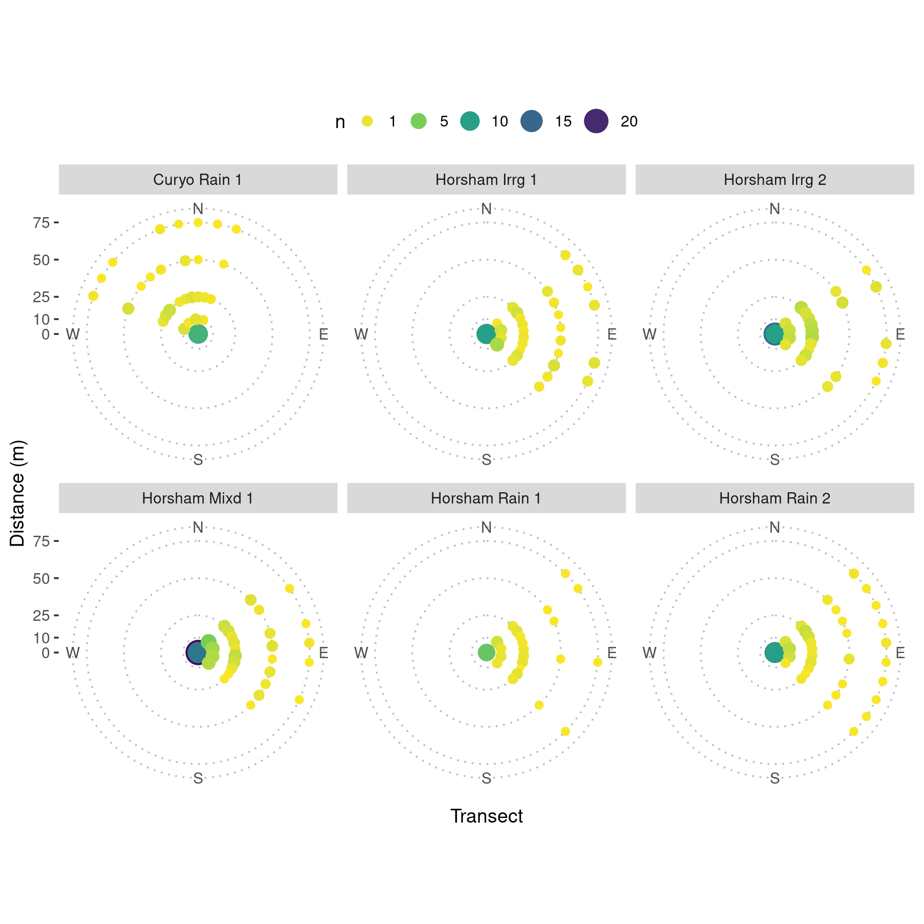

Heatmap showing count of mean lesions per plant for each pot along each of ten transects. Note that any stations where the mean count was zero for any event, the data are not shown for clarity. Events are denoted by the location, ‘Horsham’ or ‘Curyo’; source of precipitation ‘Irrg’ (irrigation), ‘Rain’ (rainfall) or ‘Mixd’ (both simultaneously); and event ‘1’, ‘2’ or ‘3.’