Fit Generalised Additive Models (GAMs) to the Dispersal Data
A.H. Sparks
2024-05-04
Source:vignettes/a05_GAM.Rmd
a05_GAM.RmdImport Data
library("ChickpeaAscoDispersal")
library("tidyverse")
library("broom")
library("ggpubr")
library("mgcv")
library("mgcViz")

theme_set(theme_pubclean(base_size = 14))
Create Data Set for GAMs
Join the lesion_counts data and the
summary_weather data to create dat for
creating GAMs.
Fit GAMs
For reproducibility purposes, use set.seed().
set.seed(27)mod1 - s(Distance)
##
## Family: gaussian
## Link function: identity
##
## Formula:
## m_lesions ~ s(distance, k = 5)
##
## Parametric coefficients:
##             Estimate Std. Error t value Pr(>|t|)
## (Intercept)  1.08024    0.04751   22.74   <2e-16 ***
## ---
## Signif. codes:  0 '***' 0.001 '**' 0.01 '*' 0.05 '.' 0.1 ' ' 1
##
## Approximate significance of smooth terms:
##               edf Ref.df    F p-value
## s(distance) 3.926  3.996 78.4  <2e-16 ***
## ---
## Signif. codes:  0 '***' 0.001 '**' 0.01 '*' 0.05 '.' 0.1 ' ' 1
##
## R-sq.(adj) =  0.482   Deviance explained = 48.8%
## GCV = 0.76522  Scale est. = 0.75394   n = 334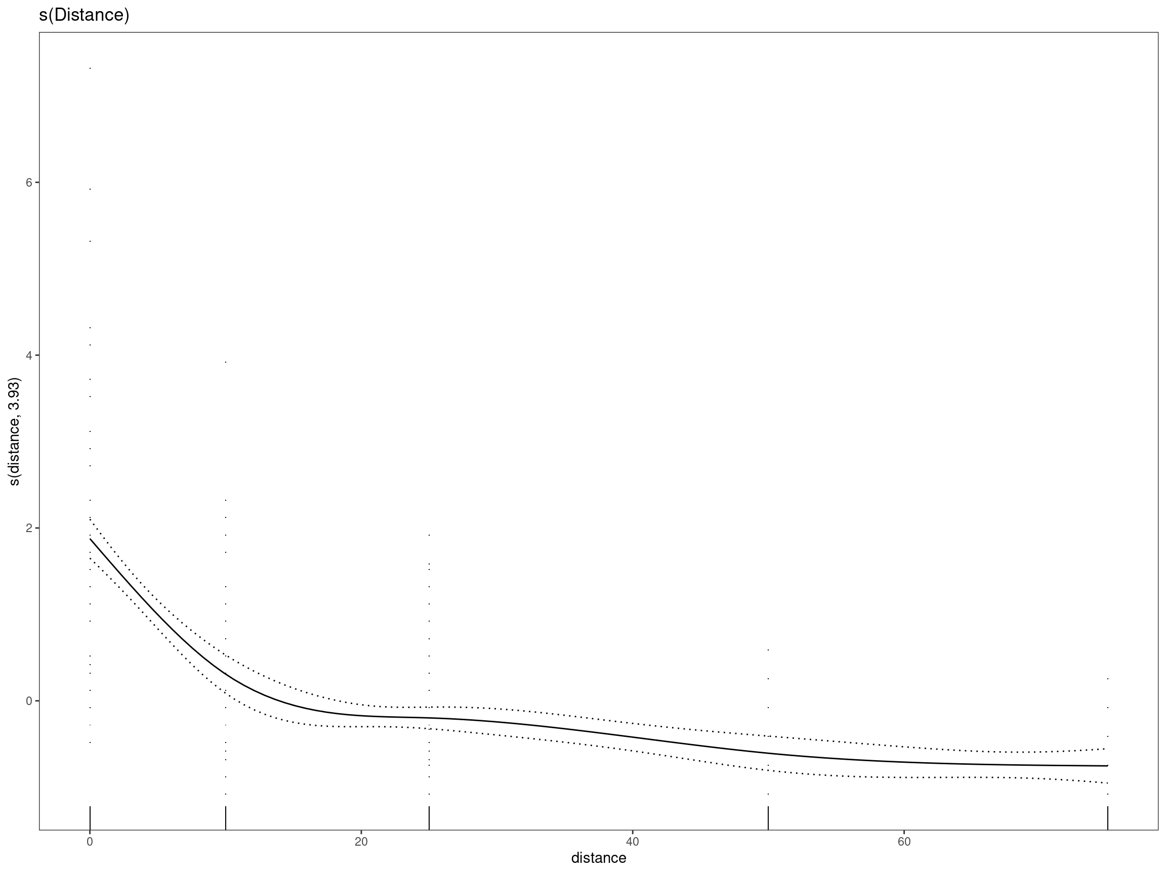
mod2 - s(Distance) + Precipitation
##
## Family: gaussian
## Link function: identity
##
## Formula:
## m_lesions ~ sum_rain + s(distance, k = 5)
##
## Parametric coefficients:
##             Estimate Std. Error t value Pr(>|t|)
## (Intercept) 0.772464   0.092471   8.354 1.89e-15 ***
## sum_rain    0.031885   0.008278   3.852 0.000141 ***
## ---
## Signif. codes:  0 '***' 0.001 '**' 0.01 '*' 0.05 '.' 0.1 ' ' 1
##
## Approximate significance of smooth terms:
##               edf Ref.df     F p-value
## s(distance) 3.928  3.996 81.76  <2e-16 ***
## ---
## Signif. codes:  0 '***' 0.001 '**' 0.01 '*' 0.05 '.' 0.1 ' ' 1
##
## R-sq.(adj) =  0.502   Deviance explained =   51%
## GCV = 0.7366  Scale est. = 0.72352   n = 334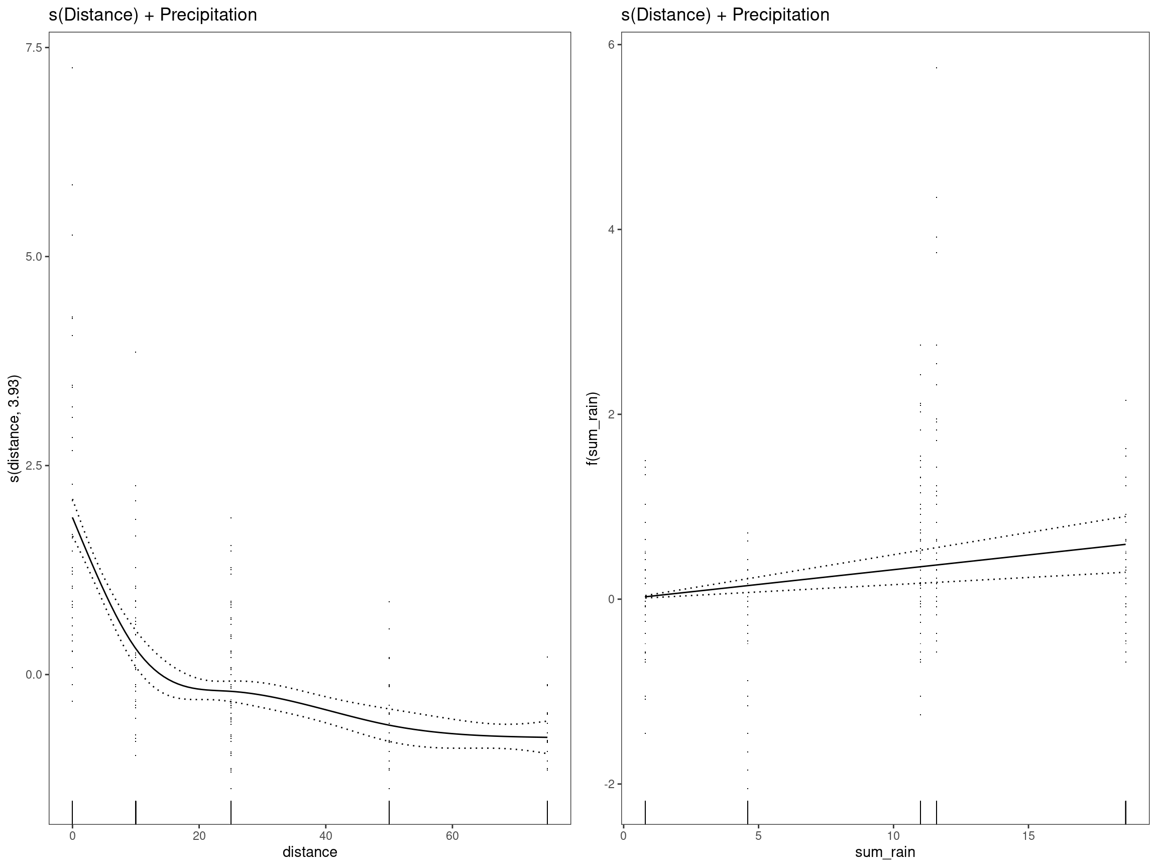
mod3 - s(Distance) + Wind speed
##
## Family: gaussian
## Link function: identity
##
## Formula:
## m_lesions ~ mws + s(distance, k = 5)
##
## Parametric coefficients:
##             Estimate Std. Error t value Pr(>|t|)
## (Intercept)  0.64401    0.11825   5.446 1.01e-07 ***
## mws          0.12273    0.03059   4.012 7.47e-05 ***
## ---
## Signif. codes:  0 '***' 0.001 '**' 0.01 '*' 0.05 '.' 0.1 ' ' 1
##
## Approximate significance of smooth terms:
##               edf Ref.df     F p-value
## s(distance) 3.929  3.996 81.99  <2e-16 ***
## ---
## Signif. codes:  0 '***' 0.001 '**' 0.01 '*' 0.05 '.' 0.1 ' ' 1
##
## R-sq.(adj) =  0.504   Deviance explained = 51.2%
## GCV = 0.73389  Scale est. = 0.72086   n = 334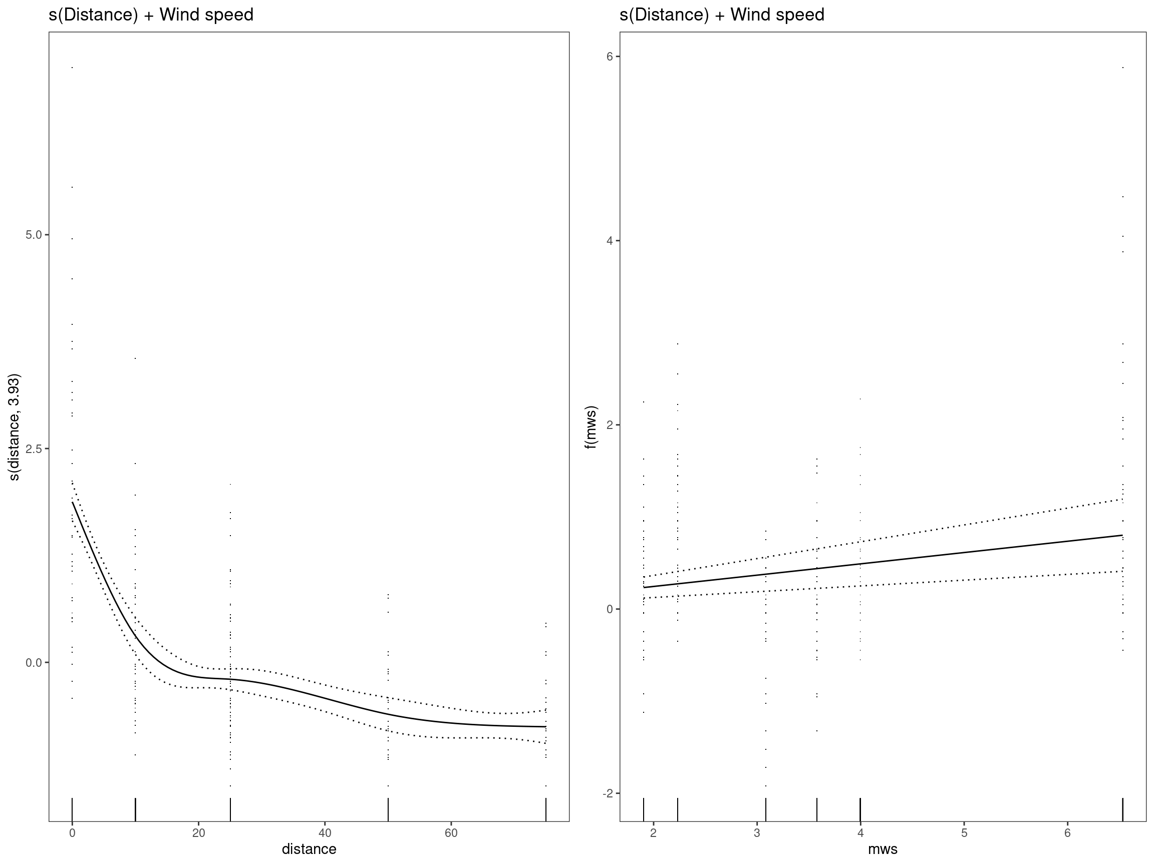
mod4 - s(Distance) + Wind speed + Precipitation
##
## Family: gaussian
## Link function: identity
##
## Formula:
## m_lesions ~ sum_rain + mws + s(distance, k = 5)
##
## Parametric coefficients:
##             Estimate Std. Error t value Pr(>|t|)
## (Intercept) 0.435675   0.132265   3.294 0.001096 **
## sum_rain    0.027392   0.008239   3.325 0.000986 ***
## mws         0.106960   0.030507   3.506 0.000518 ***
## ---
## Signif. codes:  0 '***' 0.001 '**' 0.01 '*' 0.05 '.' 0.1 ' ' 1
##
## Approximate significance of smooth terms:
##               edf Ref.df     F p-value
## s(distance) 3.931  3.996 84.56  <2e-16 ***
## ---
## Signif. codes:  0 '***' 0.001 '**' 0.01 '*' 0.05 '.' 0.1 ' ' 1
##
## R-sq.(adj) =  0.519   Deviance explained = 52.8%
## GCV = 0.71426  Scale est. = 0.69944   n = 334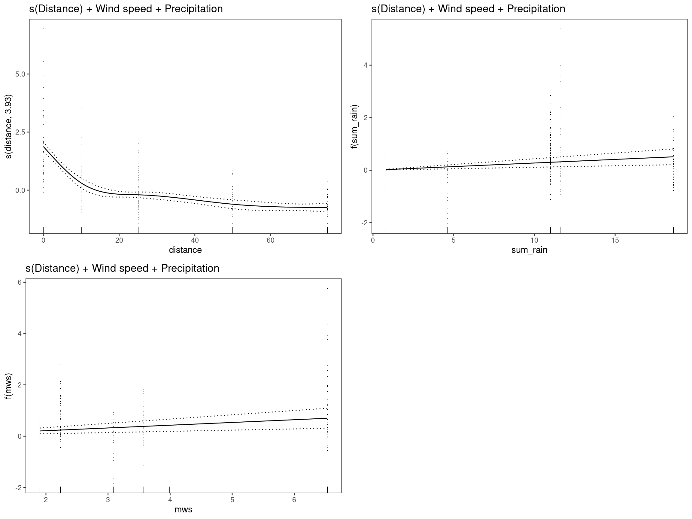
mod5 - s(Distance + Wind Speed) + Precipitation
## Warning in term[i] <- attr(terms(reformulate(term[i])), "term.labels"): number
## of items to replace is not a multiple of replacement length
summary(mod5)##
## Family: gaussian
## Link function: identity
##
## Formula:
## m_lesions ~ sum_rain + s(distance + mws, k = 5)
##
## Parametric coefficients:
## Estimate Std. Error t value Pr(>|t|)
## (Intercept) 0.772464 0.092471 8.354 1.89e-15 ***
## sum_rain 0.031885 0.008278 3.852 0.000141 ***
## ---
## Signif. codes: 0 '***' 0.001 '**' 0.01 '*' 0.05 '.' 0.1 ' ' 1
##
## Approximate significance of smooth terms:
## edf Ref.df F p-value
## s(distance) 3.928 3.996 81.76 <2e-16 ***
## ---
## Signif. codes: 0 '***' 0.001 '**' 0.01 '*' 0.05 '.' 0.1 ' ' 1
##
## R-sq.(adj) = 0.502 Deviance explained = 51%
## GCV = 0.7366 Scale est. = 0.72352 n = 334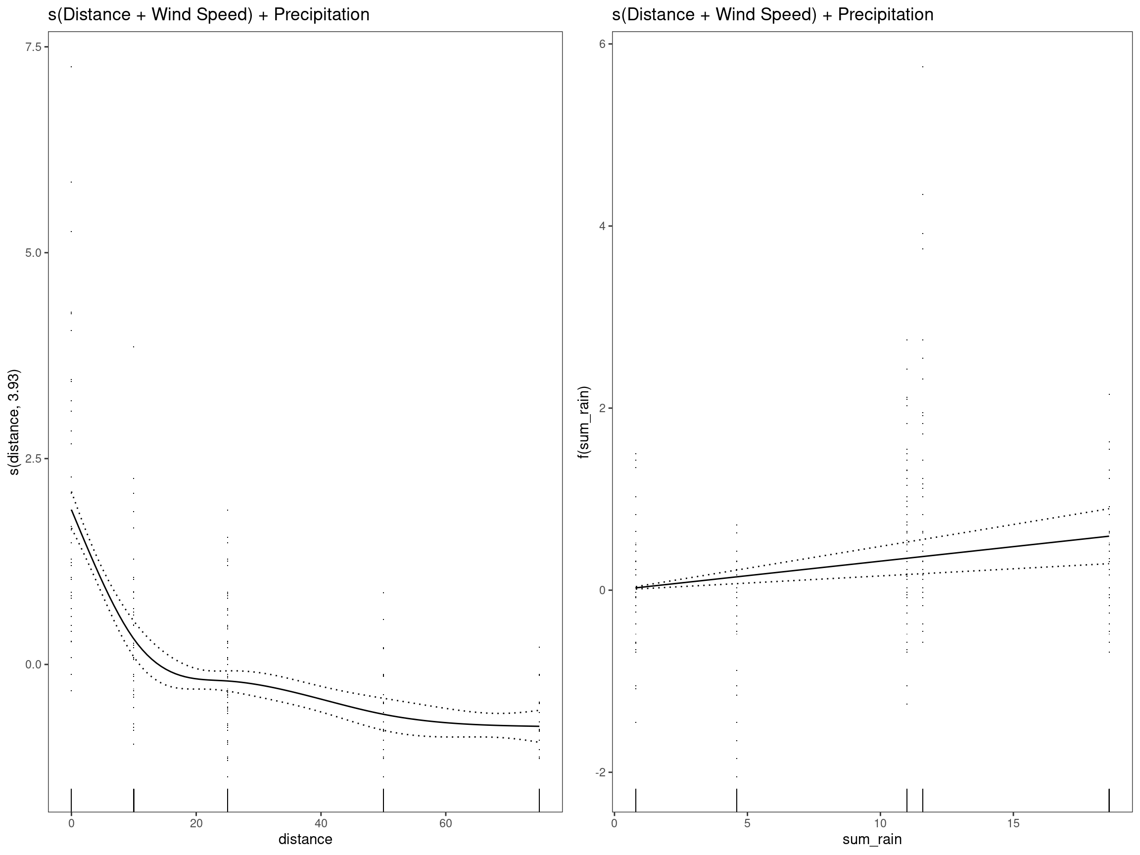
mod6 - s(Distance) + s(Wind Speed) + Precipitation
##
## Family: gaussian
## Link function: identity
##
## Formula:
## m_lesions ~ sum_rain + s(distance, k = 5) + s(mws, k = 5)
##
## Parametric coefficients:
##             Estimate Std. Error t value Pr(>|t|)
## (Intercept)  1.40355    0.18004   7.796 8.82e-14 ***
## sum_rain    -0.03349    0.01810  -1.850   0.0652 .
## ---
## Signif. codes:  0 '***' 0.001 '**' 0.01 '*' 0.05 '.' 0.1 ' ' 1
##
## Approximate significance of smooth terms:
##               edf Ref.df     F p-value
## s(distance) 3.938  3.997 93.81  <2e-16 ***
## s(mws)      3.926  3.995 12.66  <2e-16 ***
## ---
## Signif. codes:  0 '***' 0.001 '**' 0.01 '*' 0.05 '.' 0.1 ' ' 1
##
## R-sq.(adj) =  0.566   Deviance explained = 57.8%
## GCV = 0.6497  Scale est. = 0.63051   n = 334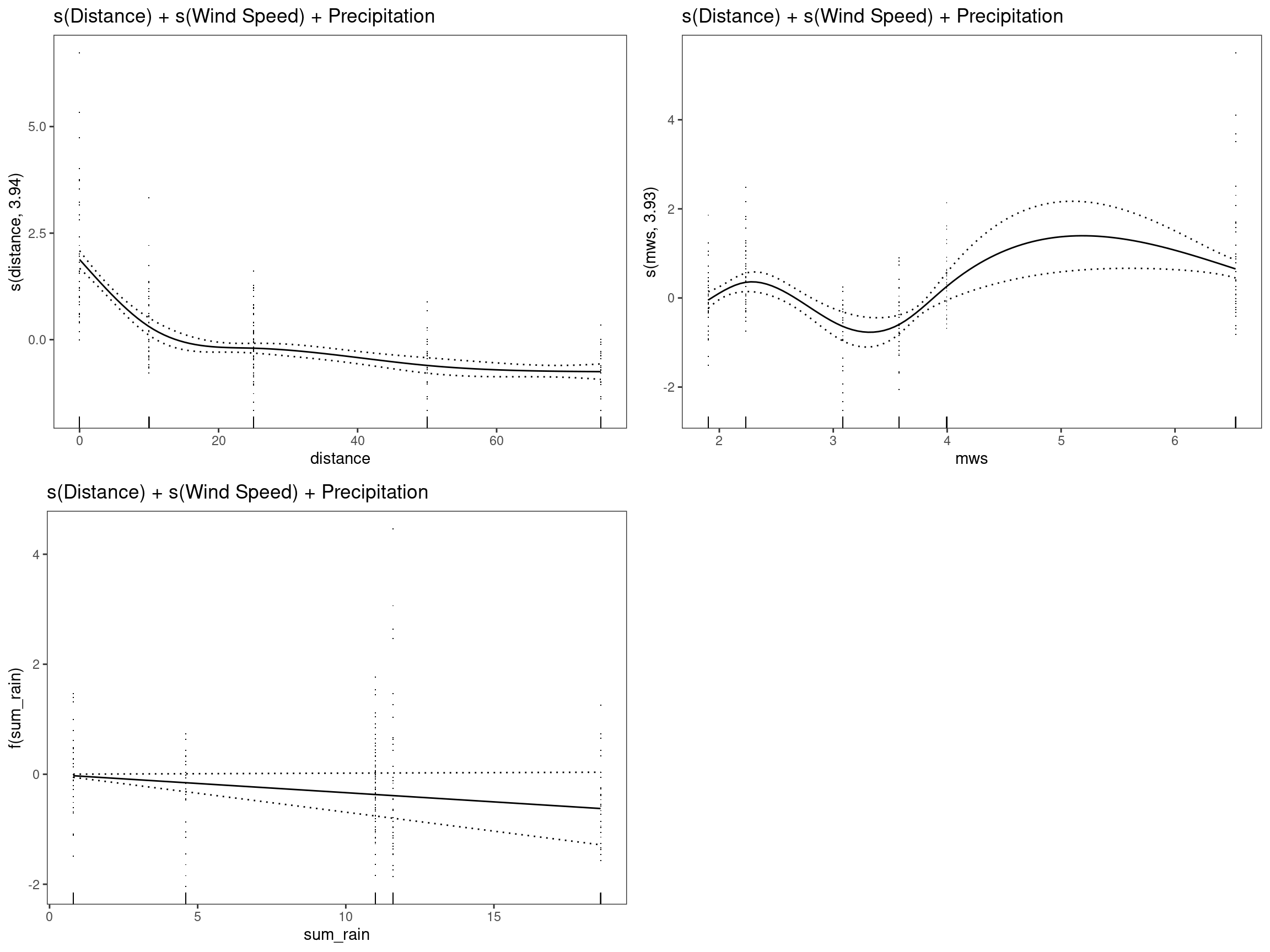
mod7 - s(Distance) + s(Wind Speed)
##
## Family: gaussian
## Link function: identity
##
## Formula:
## m_lesions ~ s(distance, k = 5) + s(mws, k = 5)
##
## Parametric coefficients:
##             Estimate Std. Error t value Pr(>|t|)
## (Intercept)  1.08024    0.04366   24.74   <2e-16 ***
## ---
## Signif. codes:  0 '***' 0.001 '**' 0.01 '*' 0.05 '.' 0.1 ' ' 1
##
## Approximate significance of smooth terms:
##               edf Ref.df     F p-value
## s(distance) 3.937  3.997 92.96  <2e-16 ***
## s(mws)      3.917  3.995 16.04  <2e-16 ***
## ---
## Signif. codes:  0 '***' 0.001 '**' 0.01 '*' 0.05 '.' 0.1 ' ' 1
##
## R-sq.(adj) =  0.562   Deviance explained = 57.3%
## GCV = 0.65392  Scale est. = 0.63659   n = 334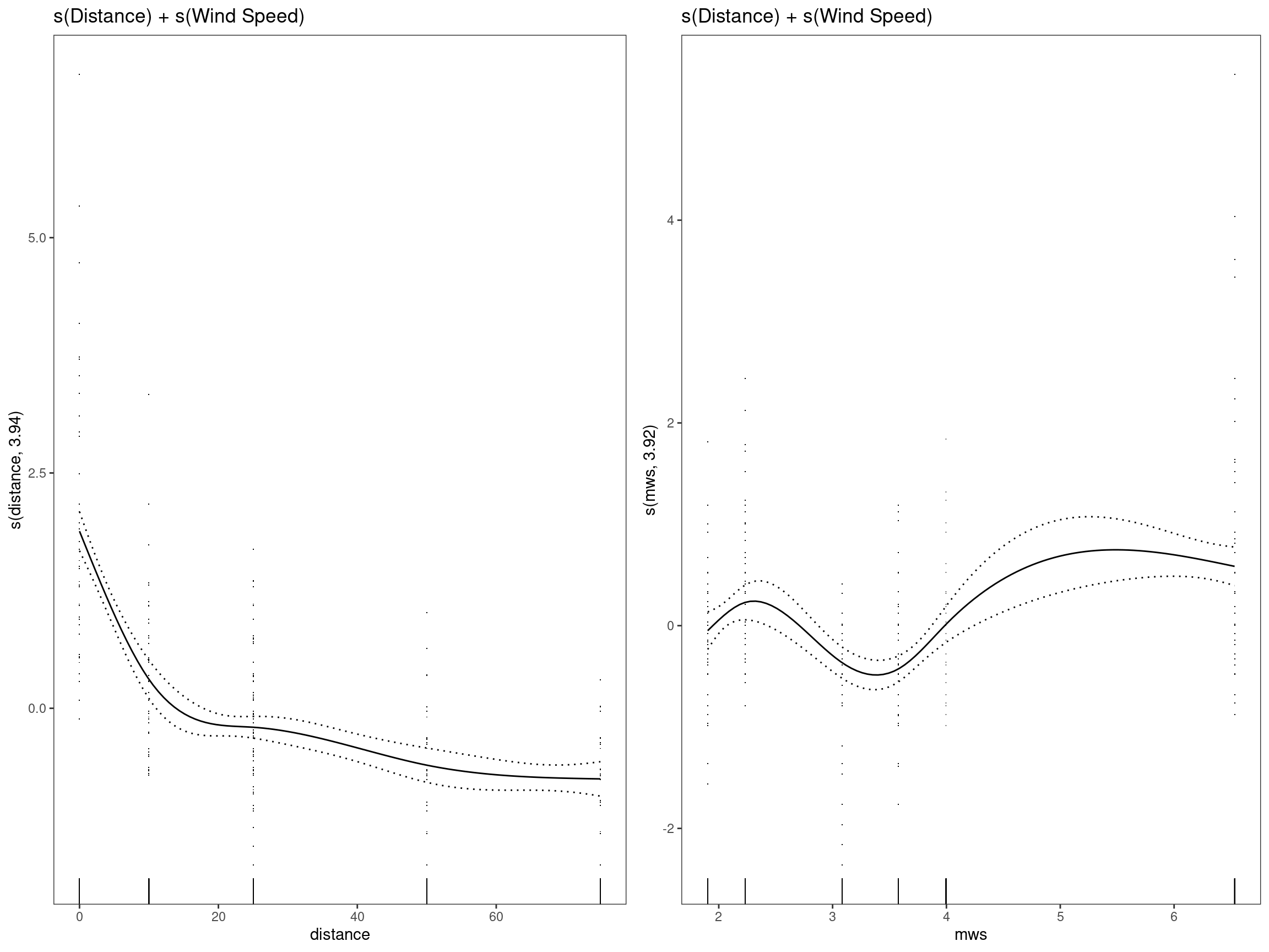
mod8 - s(Distance) + s(Wind Speed) + s(Precipitation)
mod8 <-
   gam(
      m_lesions ~ s(distance, k = 5) + s(mws, k = 5) + s(sum_rain, k = 5),
      data = dat
   )

summary(mod8)
##
## Family: gaussian
## Link function: identity
##
## Formula:
## m_lesions ~ s(distance, k = 5) + s(mws, k = 5) + s(sum_rain,
## k = 5)
##
## Parametric coefficients:
## Estimate Std. Error t value Pr(>|t|)
## (Intercept) 1.08024 0.04345 24.86 <2e-16 ***
## ---
## Signif. codes: 0 '***' 0.001 '**' 0.01 '*' 0.05 '.' 0.1 ' ' 1
##
## Approximate significance of smooth terms:
## edf Ref.df F p-value
## s(distance) 3.938 3.997 93.805 <2e-16 ***
## s(mws) 1.666 1.761 1.356 0.3404
## s(sum_rain) 3.192 3.219 3.298 0.0113 *
## ---
## Signif. codes: 0 '***' 0.001 '**' 0.01 '*' 0.05 '.' 0.1 ' ' 1
##
## R-sq.(adj) = 0.566 Deviance explained = 57.8%
## GCV = 0.64956 Scale est. = 0.63051 n = 334
print(p_gam(x = getViz(mod8)) +
         ggtitle("s(Distance) + s(Wind Speed) + s(Precipitation)"),
      pages = 1)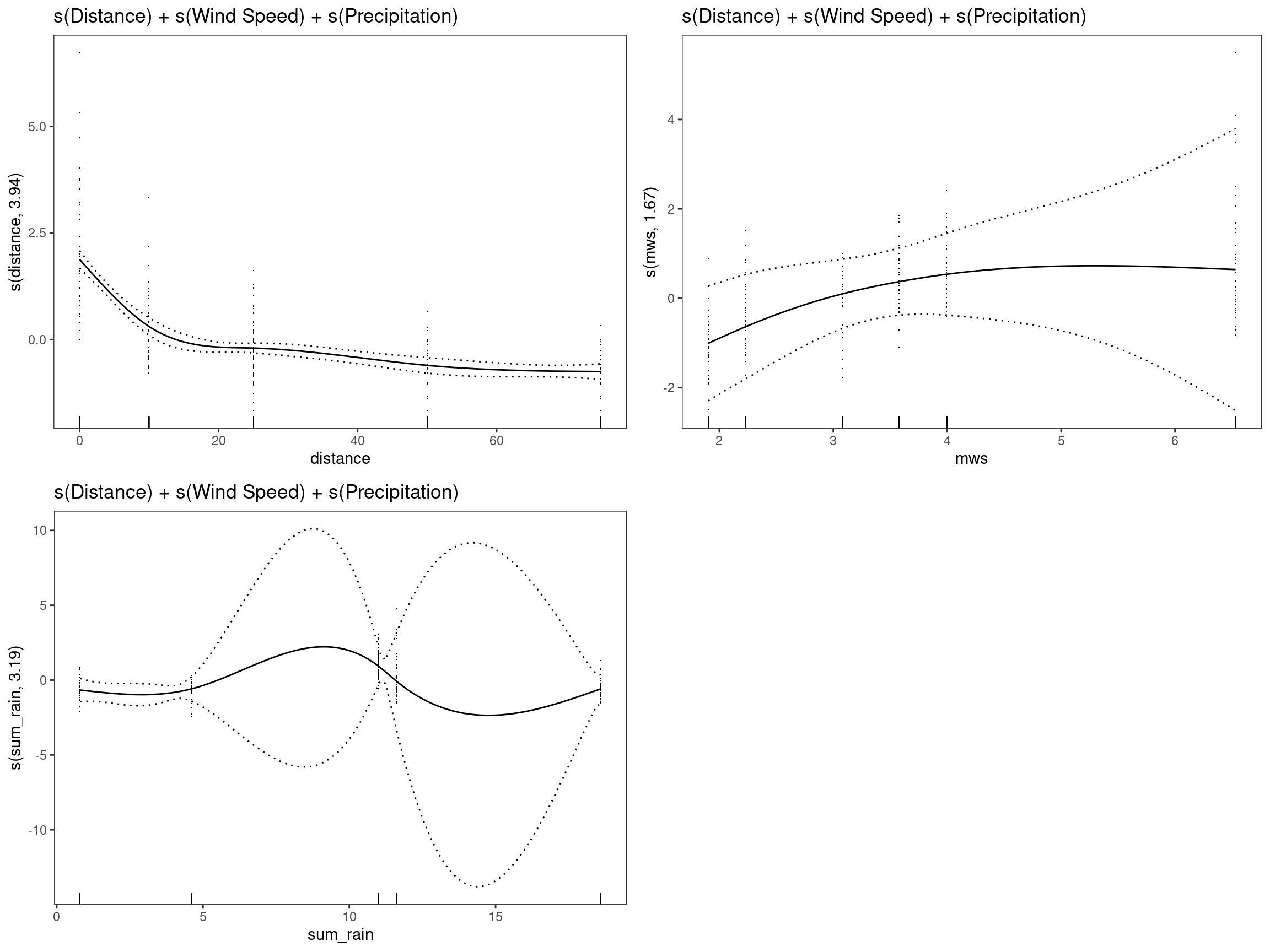
mod9 - s(Distance) + s(Precipitation)
##
## Family: gaussian
## Link function: identity
##
## Formula:
## m_lesions ~ s(distance, k = 5) + s(sum_rain, k = 5)
##
## Parametric coefficients:
##             Estimate Std. Error t value Pr(>|t|)
## (Intercept)  1.08024    0.04393   24.59   <2e-16 ***
## ---
## Signif. codes:  0 '***' 0.001 '**' 0.01 '*' 0.05 '.' 0.1 ' ' 1
##
## Approximate significance of smooth terms:
##               edf Ref.df     F p-value
## s(distance) 3.936  3.997 91.78  <2e-16 ***
## s(sum_rain) 3.901  3.991 15.19  <2e-16 ***
## ---
## Signif. codes:  0 '***' 0.001 '**' 0.01 '*' 0.05 '.' 0.1 ' ' 1
##
## R-sq.(adj) =  0.557   Deviance explained = 56.7%
## GCV = 0.66195  Scale est. = 0.64444   n = 334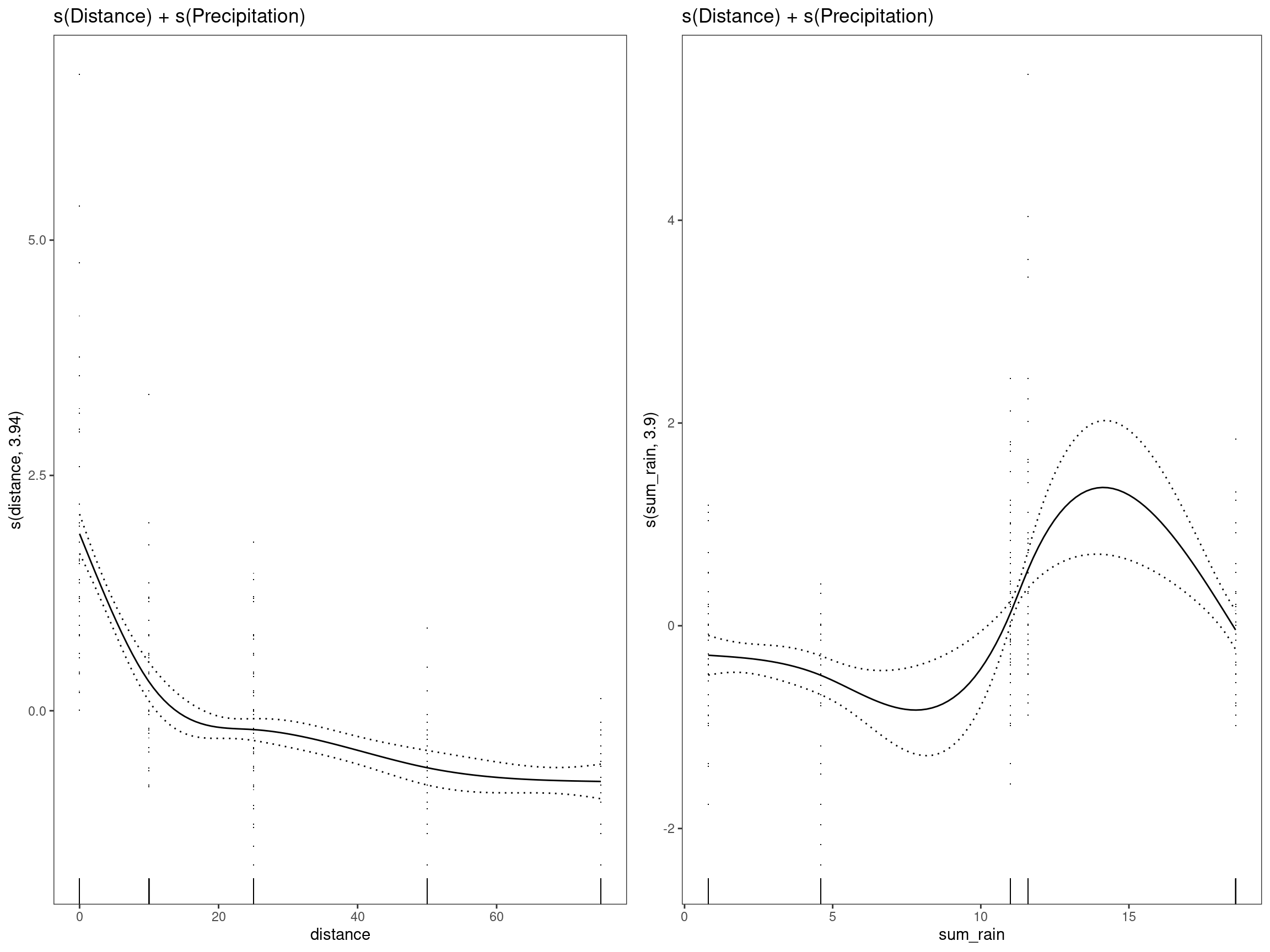
mod10 - s(Distance) +s(Precipitation) + Wind speed
mod10 <-
   gam(
      m_lesions ~ s(distance, k = 5) + s(sum_rain, k = 5) + mws,
      data = dat
   )

summary(mod10)
##
## Family: gaussian
## Link function: identity
##
## Formula:
## m_lesions ~ s(distance, k = 5) + s(sum_rain, k = 5) + mws
##
## Parametric coefficients:
## Estimate Std. Error t value Pr(>|t|)
## (Intercept) -2.5358 1.4136 -1.794 0.0738 .
## mws 1.0174 0.3975 2.559 0.0109 *
## ---
## Signif. codes: 0 '***' 0.001 '**' 0.01 '*' 0.05 '.' 0.1 ' ' 1
##
## Approximate significance of smooth terms:
## edf Ref.df F p-value
## s(distance) 3.937 3.997 93.76 <2e-16 ***
## s(sum_rain) 3.764 3.944 13.68 <2e-16 ***
## ---
## Signif. codes: 0 '***' 0.001 '**' 0.01 '*' 0.05 '.' 0.1 ' ' 1
##
## R-sq.(adj) = 0.566 Deviance explained = 57.8%
## GCV = 0.64968 Scale est. = 0.63081 n = 334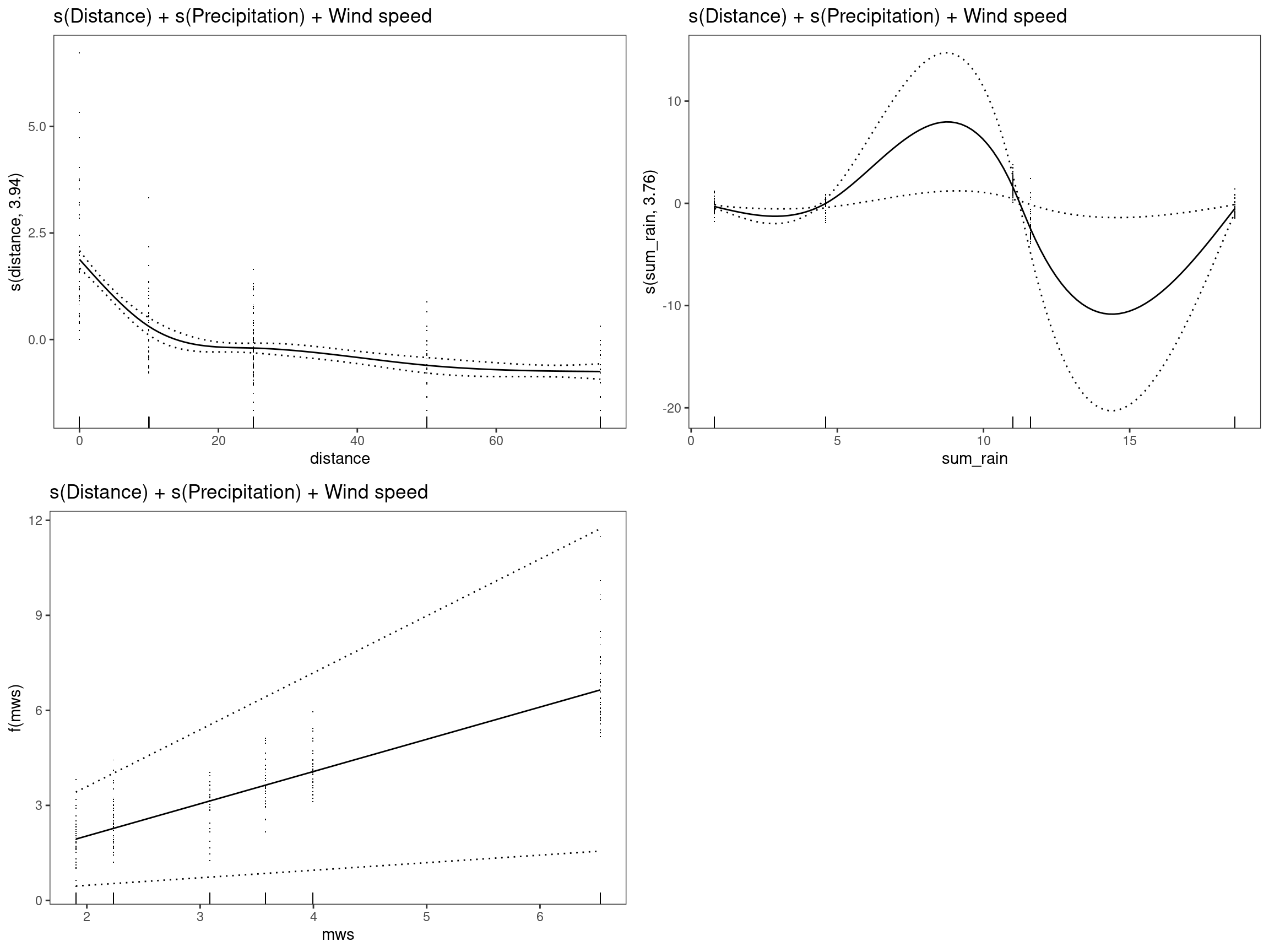
mod11 - s(Distance) + s(Wind Speed) + s(Precipitation), family = tw()
This is the same as mod8 but using
family = tw(), see ?family.mgcv for more on
the families. The Tweedie distribution is used where the distribution
has a positive mass at zero, but is continuous unlike the Poisson
distribution that requires count data. The data visualisation shows
clearly that the mean pot count data have this shape.
mod11 <-
   gam(
      m_lesions ~ s(distance, k = 5) +
         s(mws, k = 5) +
         s(sum_rain, k = 5),
      data = dat,
      family = tw()
   )

summary(mod11)
##
## Family: Tweedie(p=1.044)
## Link function: log
##
## Formula:
## m_lesions ~ s(distance, k = 5) + s(mws, k = 5) + s(sum_rain,
## k = 5)
##
## Parametric coefficients:
## Estimate Std. Error t value Pr(>|t|)
## (Intercept) -0.22823 0.04098 -5.569 5.39e-08 ***
## ---
## Signif. codes: 0 '***' 0.001 '**' 0.01 '*' 0.05 '.' 0.1 ' ' 1
##
## Approximate significance of smooth terms:
## edf Ref.df F p-value
## s(distance) 3.496 3.855 123.776 < 2e-16 ***
## s(mws) 1.992 2.092 0.824 0.45080
## s(sum_rain) 2.812 2.879 5.493 0.00168 **
## ---
## Signif. codes: 0 '***' 0.001 '**' 0.01 '*' 0.05 '.' 0.1 ' ' 1
##
## R-sq.(adj) = 0.674 Deviance explained = 61.2%
## -REML = 309.96 Scale est. = 0.36397 n = 334
print(p_gam(x = getViz(mod11)) +
   ggtitle("s(Distance) + s(Wind Speed) + s(Precipitation), family = tw()"),
   pages = 1)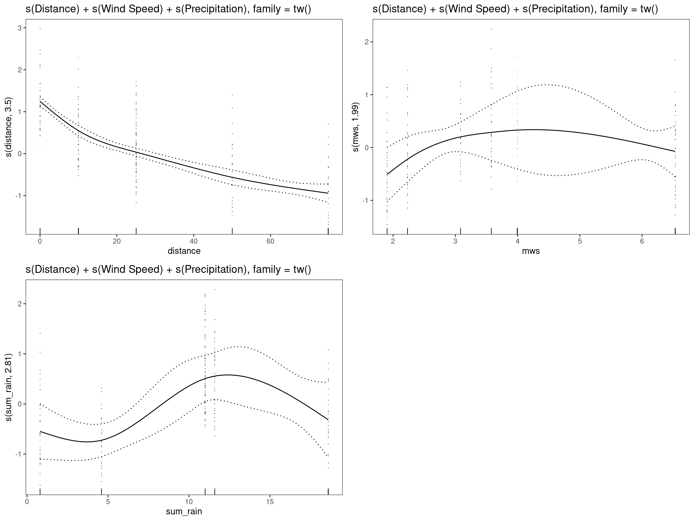
mod12 - s(Distance, bs = “ts”) + s(Precipitation, bs = “ts”) Wind speed, family = tw()
Try using wind speed as a linear predictor only.
mod12 <-
   gam(
      m_lesions ~ s(distance, k = 5, bs = "ts") +
         s(mws, k = 5, bs = "ts") +
         s(sum_rain, k = 5, bs = "ts"),
      data = dat,
      family = tw()
   )

summary(mod12)
##
## Family: Tweedie(p=1.044)
## Link function: log
##
## Formula:
## m_lesions ~ s(distance, k = 5, bs = "ts") + s(mws, k = 5, bs = "ts") +
## s(sum_rain, k = 5, bs = "ts")
##
## Parametric coefficients:
## Estimate Std. Error t value Pr(>|t|)
## (Intercept) -0.22200 0.04089 -5.43 1.11e-07 ***
## ---
## Signif. codes: 0 '***' 0.001 '**' 0.01 '*' 0.05 '.' 0.1 ' ' 1
##
## Approximate significance of smooth terms:
## edf Ref.df F p-value
## s(distance) 3.2481 4 117.664 < 2e-16 ***
## s(mws) 0.9088 4 2.403 0.00027 ***
## s(sum_rain) 2.8645 4 15.752 < 2e-16 ***
## ---
## Signif. codes: 0 '***' 0.001 '**' 0.01 '*' 0.05 '.' 0.1 ' ' 1
##
## R-sq.(adj) = 0.657 Deviance explained = 60%
## -REML = 319.36 Scale est. = 0.36504 n = 334
print(
   p_gam(x = getViz(mod12)) +
      ggtitle(
         "s(Distance, bs = 'ts') + s(Wind speed, bs = 'ts')\n+ s(Precipitation, bs = 'ts'), family = tw()"
      ),
   pages = 1
)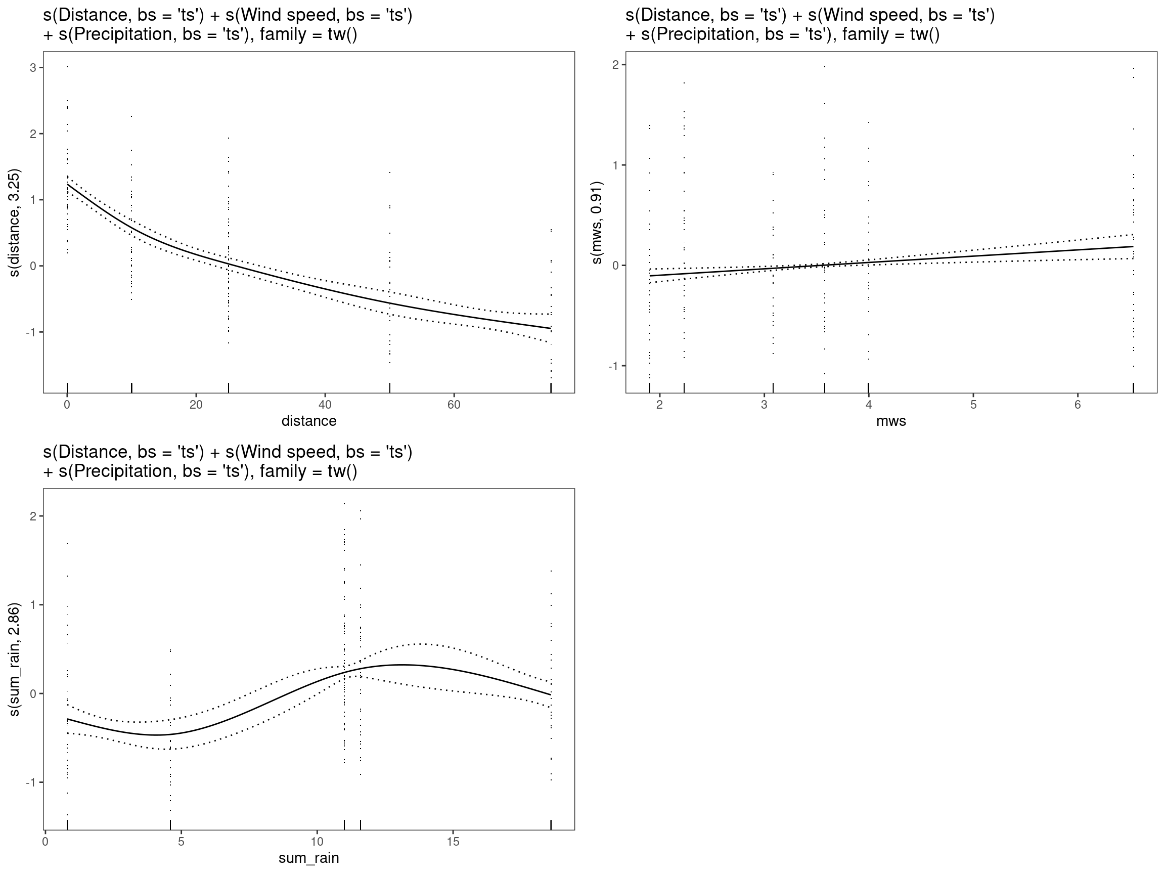
mod13 - s(Distance, bs = “ts”) + s(Wind speed, bs = “ts”) + s(Precipitation, bs = “ts”), family = tw()
mod13 <-
   gam(
      m_lesions ~ s(distance, k = 5, bs = "ts") +
         s(mws, k = 5, bs = "ts") +
         s(sum_rain, k = 5, bs = "ts"),
      data = dat,
      family = tw()
   )

summary(mod13)
##
## Family: Tweedie(p=1.044)
## Link function: log
##
## Formula:
## m_lesions ~ s(distance, k = 5, bs = "ts") + s(mws, k = 5, bs = "ts") +
## s(sum_rain, k = 5, bs = "ts")
##
## Parametric coefficients:
## Estimate Std. Error t value Pr(>|t|)
## (Intercept) -0.22200 0.04089 -5.43 1.11e-07 ***
## ---
## Signif. codes: 0 '***' 0.001 '**' 0.01 '*' 0.05 '.' 0.1 ' ' 1
##
## Approximate significance of smooth terms:
## edf Ref.df F p-value
## s(distance) 3.2481 4 117.664 < 2e-16 ***
## s(mws) 0.9088 4 2.403 0.00027 ***
## s(sum_rain) 2.8645 4 15.752 < 2e-16 ***
## ---
## Signif. codes: 0 '***' 0.001 '**' 0.01 '*' 0.05 '.' 0.1 ' ' 1
##
## R-sq.(adj) = 0.657 Deviance explained = 60%
## -REML = 319.36 Scale est. = 0.36504 n = 334
print(
   p_gam(x = getViz(mod13)) +
      ggtitle(
         "s(Distance, bs = 'ts') + s(Wind speed, bs = 'ts')\n+ s(Precipitation, bs = 'ts'), family = tw()"
      ),
   pages = 1
)
This model, same structure as mod11, uses thin-plate
splines to shrink the coefficients of the smooth to zero when
possible.
Compare the Models
AIC, BIC
models <- list(mod1 = mod1,
               mod2 = mod2,
               mod3 = mod3,
               mod4 = mod4,
               mod5 = mod5,
               mod6 = mod6,
               mod7 = mod7,
               mod8 = mod8,
               mod9 = mod9,
               mod10 = mod10,
               mod11 = mod11,
               mod12 = mod12,
               mod13 = mod13
               )
map_df(models, glance, .id = "model") %>%
   arrange(AIC)
## # A tibble: 13 × 8
## model df logLik AIC BIC deviance df.residual nobs
## <chr> <dbl> <dbl> <dbl> <dbl> <dbl> <dbl> <int>
## 1 mod11 9.30 -288. 599. 644. 141. 325. 334
## 2 mod12 8.02 -293. 608. 649. 145. 326. 334
## 3 mod13 8.02 -293. 608. 649. 145. 326. 334
## 4 mod8 9.80 -392. 805. 847. 204. 324. 334
## 5 mod10 9.70 -392. 806. 846. 205. 324. 334
## 6 mod6 9.86 -392. 806. 847. 204. 324. 334
## 7 mod7 8.85 -394. 808. 845. 207. 325. 334
## 8 mod9 8.84 -396. 812. 849. 210. 325. 334
## 9 mod4 6.93 -411. 837. 868. 229. 327. 334
## 10 mod3 5.93 -416. 846. 873. 236. 328. 334
## 11 mod2 5.93 -417. 848. 874. 237. 328. 334
## 12 mod5 5.93 -417. 848. 874. 237. 328. 334
## 13 mod1 4.93 -424. 860. 883. 248. 329. 334R2
enframe(c(
   mod1 = summary(mod1)$r.sq,
   mod2 = summary(mod2)$r.sq,
   mod3 = summary(mod3)$r.sq,
   mod4 = summary(mod4)$r.sq,
   mod5 = summary(mod5)$r.sq,
   mod6 = summary(mod6)$r.sq,
   mod7 = summary(mod7)$r.sq,
   mod8 = summary(mod8)$r.sq,
   mod9 = summary(mod9)$r.sq,
   mod10 = summary(mod10)$r.sq,
   mod11 = summary(mod11)$r.sq,
   mod12 = summary(mod12)$r.sq,
   mod13 = summary(mod13)$r.sq
)) %>%
   arrange(desc(value))
## # A tibble: 13 × 2
## name value
## <chr> <dbl>
## 1 mod11 0.674
## 2 mod12 0.657
## 3 mod13 0.657
## 4 mod8 0.566
## 5 mod6 0.566
## 6 mod10 0.566
## 7 mod7 0.562
## 8 mod9 0.557
## 9 mod4 0.519
## 10 mod3 0.504
## 11 mod2 0.502
## 12 mod5 0.502
## 13 mod1 0.482NOTE The original work had an
anova.gam()to compare the models. Somehow, somewhere it seems that changes have been made and current versions of the R packages don’t allow an ANOVA comparison for GAMs that usefamily = tw(), so this portion has been removed from this vignette. -ahs 2024-04-28
Check Best Model Fit
mod11 - s(Distance) + s(Wind Speed) + s(Precipitation), family = tw()
mod11_vis <- getViz(mod11)
check(mod11_vis,
      a.qq = list(method = "tnorm",
                  a.cipoly = list(fill = "light blue")),
      a.respoi = list(size = 0.5),
      a.hist = list(bins = 10))
##
## Method: REML Optimizer: outer newton
## full convergence after 8 iterations.
## Gradient range [-4.288874e-07,2.610557e-07]
## (score 309.9554 & scale 0.3639671).
## Hessian positive definite, eigenvalue range [0.3685077,2978.832].
## Model rank = 13 / 13
##
## Basis dimension (k) checking results. Low p-value (k-index<1) may
## indicate that k is too low, especially if edf is close to k'.
##
## k' edf k-index p-value
## s(distance) 4.00 3.50 0.87 0.02 *
## s(mws) 4.00 1.99 0.98 0.51
## s(sum_rain) 4.00 2.81 1.00 0.65
## ---
## Signif. codes: 0 '***' 0.001 '**' 0.01 '*' 0.05 '.' 0.1 ' ' 1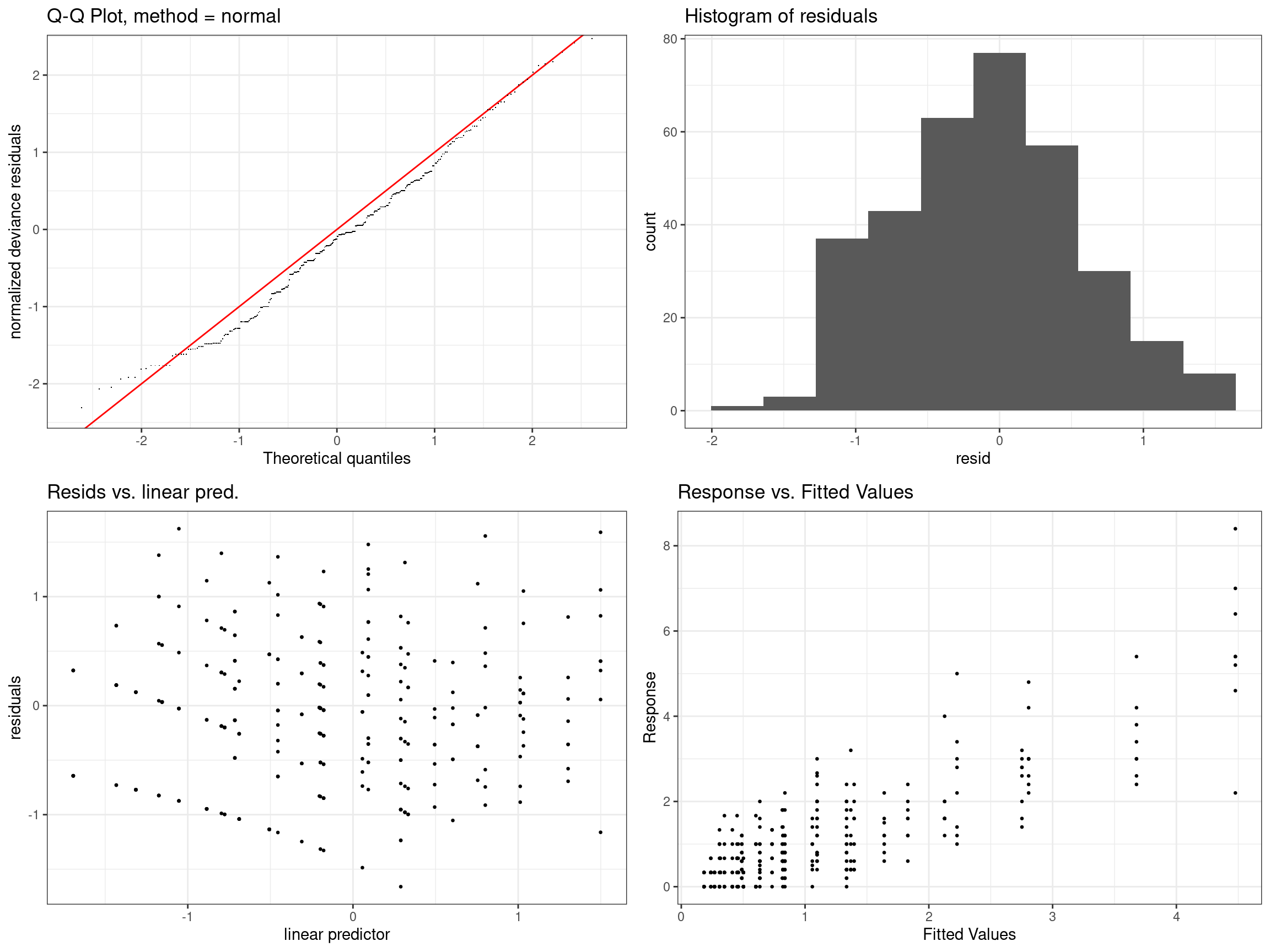
# generate a new plot.gam object just for the publication (no main title)
p11 <- p_gam(x = getViz(mod11))

# save png and eps files
png(
   file = here::here("man/figures", "Fig1.png"),
   width = 640,
   height = 640,
   units = "px",
   pointsize = 14
)
print(p11, pages = 1)
dev.off()

postscript(file = here::here("man/figures", "Fig1.eps"),
           family = "Arial")
par(mar = c(5, 3, 2, 2) + 0.1)
print(p11, pages = 1)
dev.off()

embed_fonts(
   file = here::here("man/figures", "Fig1.eps"),
   outfile = here::here("man/figures", "Fig1.eps"),
   options = "-dEPSCrop"
)
Thoughts
This model, mod11,
m_lesions ~ s(Distance) + s(WindSpeed) + s(Precipitation) - family = tw(),
is the best performing model. It cannot be used for predictions, but
suitably describes the dispersal data we have on hand with the
parameters used. More data would be desirable to increase the value of
k as evidenced in the GAM checks.