Working with spatial data available through read.abares
Adam H. Sparks
2025-12-14
Source:vignettes/read.abares.Rmd
read.abares.RmdThis vignette demonstrates some of the functionality of {read.abares} and how to work with some of the spatial and tabular data available through {read.abares}. Please note that not all functions are demonstrated here, please refer to the function reference documentation for a full list of functionality. The worked examples here show some of the more advanced features that {read.abares} offers beyond just fetching and importing data, e.g., Australian Agricultural and Grazing Industries Survey (AAGIS) spatial shapefile which can be used with tabular data from the historical estimates, the Australian Gridded Farm Data, which can be downloaded and imported using one of four types of object or the soil thickness data, which includes rich metadata.
First we need to load the {read.abares} library.
library(read.abares)
#>
#> Attaching package: 'read.abares'
#> The following object is masked from 'package:graphics':
#>
#>     plot
#> The following objects are masked from 'package:base':
#>
#>     levels, plot
Working with AAGIS Regions Spatial Data
Obtaining the AAGIS Regions Spatial Data
ABARES offers spatial data for the Australian Agricultural and
Grazing Industries Survey (AAGIS) regions that can be used for mapping
tabular data from the estimates, e.g.,
read_historical_regional_estimates() or
read_state_estimates().
aagis_regions <- read_aagis_regions()

plot(aagis_regions)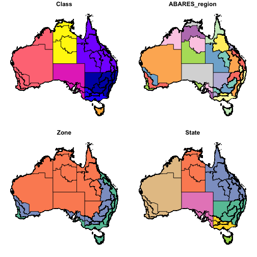
AAGIS regions shapefile
Obtaining AAGIS Data by Region
{read.abares} offers functions to download the ABARES estimates based
on the AAGIS results for national level,
read_historical_national_estimates(), regional level
read_historical_regional_estimates(), and state level
read_historical_state_estimates() and also by performance
category read_estimates_by_performance_category() and size
category read_estimates_by_size(). For this example, we
will use the read_historical_regional_estimates() function
to download the AAGIS data for the regions in the AAGIS regions
shapefile and join the data and visualise some of the data.
aagis_region_data <- read_historical_regional_estimates()
#>   OpenMP version (_OPENMP)       201811
#>   omp_get_num_procs()            10
#>   R_DATATABLE_NUM_PROCS_PERCENT  unset (default 50)
#>   R_DATATABLE_NUM_THREADS        unset
#>   R_DATATABLE_THROTTLE           unset (default 1024)
#>   omp_get_thread_limit()         2147483647
#>   omp_get_max_threads()          10
#>   OMP_THREAD_LIMIT               unset
#>   OMP_NUM_THREADS                unset
#>   RestoreAfterFork               true
#>   data.table is using 5 threads with throttle==1024. See ?setDTthreads.
#> freadR.c has been passed a filename: /var/folders/vz/txwj1tx51txgw7zv_b5c5_3m0000gn/T/Rtmp5Uncbj/fdp-beta-regional-historical.csv
#> [01] Check arguments
#>   Using 5 threads (omp_get_max_threads()=10, nth=5)
#>   NAstrings = [<<NA>>]
#>   None of the NAstrings look like numbers.
#>   show progress = 1
#>   0/1 column will be read as integer
#>   Y/N column will be read as character
#> [02] Opening the file
#>   Opening file /var/folders/vz/txwj1tx51txgw7zv_b5c5_3m0000gn/T/Rtmp5Uncbj/fdp-beta-regional-historical.csv
#>   File opened, size = 9.39MB (9846892 bytes).
#>   Memory mapped ok
#> [03] Detect and skip BOM
#> [04] Arrange mmap to be \0 terminated
#>   \n has been found in the input and different lines can end with different line endings (e.g. mixed \n and \r\n in one file). This is common and ideal.
#> [05] Skipping initial rows if needed
#>   Positioned on line 1 starting: <<Variable,Year,ABARES region,Va>>
#> [06] Detect separator, quoting rule, and ncolumns
#>   Detecting sep automatically ...
#>   sep=','  with 100 lines of 5 fields using quote rule 0
#>   Detected 5 columns on line 1. This line is either column names or first data row. Line starts as: <<Variable,Year,ABARES region,Va>>
#>   Quote rule picked = 0
#>   fill=false and the most number of columns found is 5
#> [07] Detect column types, dec, good nrow estimate and whether first row is column names
#>   sep=',' so dec set to '.'
#>   Number of sampling jump points = 100 because (9846891 bytes from row 1 to eof) / (2 * 5835 jump0size) == 843
#>   Type codes (jump 000)    : E7E99  Quote rule 0
#>   Type codes (jump 100)    : E7E99  Quote rule 0
#>   'header' determined to be true due to column 2 containing a string on row 1 and a lower type (int32) in the rest of the 10052 sample rows
#>   =====
#>   Sampled 10052 rows (handled \n inside quoted fields) at 101 jump points
#>   Bytes from first data row on line 2 to the end of last row: 9846853
#>   Line length: mean=66.42 sd=13.33 min=33 max=123
#>   Estimated number of rows: 9846853 / 66.42 = 148252
#>   Initial alloc = 247691 rows (148252 + 67%) using bytes/max(mean-2*sd,min) clamped between [1.1*estn, 2.0*estn]
#>   =====
#> [08] Assign column names
#> [09] Apply user overrides on column types
#>   After 0 type and 0 drop user overrides : E7E99
#> [10] Allocate memory for the datatable
#>   Allocating 5 column slots (5 - 0 dropped) with 247691 rows
#> [11] Read the data
#>   jumps=[0..10), chunk_size=984685, total_size=9846853
#> Read 150480 rows x 5 columns from 9.39MB (9846892 bytes) file in 00:00.011 wall clock time
#> [12] Finalizing the datatable
#>   Type counts:
#>          1 : int32     '7'
#>          2 : float64   '9'
#>          2 : string    'E'
#> =============================
#>    0.000s (  4%) Memory map 0.009GB file
#>    0.001s (  9%) sep=',' ncol=5 and header detection
#>    0.000s (  0%) Column type detection using 10052 sample rows
#>    0.000s (  1%) Allocation of 247691 rows x 5 cols (0.008GB) of which 150480 ( 61%) rows used
#>    0.010s ( 85%) Reading 10 chunks (0 swept) of 0.939MB (each chunk 15048 rows) using 5 threads
#>    +    0.002s ( 17%) Parse to row-major thread buffers (grown 0 times)
#>    +    0.005s ( 41%) Transpose
#>    +    0.003s ( 28%) Waiting
#>    0.000s (  0%) Rereading 0 columns due to out-of-sample type exceptions
#>    0.011s        Total
Filter the AAGIS region data to represent the total area cropped for the year of 2023. This will make the next few examples execute much more quickly.
library(dplyr)
#>
#> Attaching package: 'dplyr'
#> The following objects are masked from 'package:stats':
#>
#>     filter, lag
#> The following objects are masked from 'package:base':
#>
#>     intersect, setdiff, setequal, union

aagis_region_data <- filter(aagis_region_data,
                            Variable == "Total area cropped (ha)",
                            Year == 2023)
Merging the AAGIS Regions Spatial Data with the AAGIS Regional Data
Using read_aagis_regions() and
read_historical_regional_estimates(), we can merge the two
datasets together to visualise the data. To join the data, we will use
the left_join() function from the {dplyr} package.
aagis_dat <- left_join(aagis_regions, aagis_region_data)
#> Joining with `by = join_by(ABARES_region)`
Once we’ve joined the data, we can visualise it using {ggplot2}. Here we can plot the total area cropped (ha) for all of Australia for the year 2023.
library(ggplot2)

ggplot(aagis_dat) +
  geom_sf(aes(fill = Value), colour = NA) +
  scale_fill_viridis_c() +
  labs(
    fill = "Total Area Cropped (ha)"
  ) +
  facet_wrap(~Year) +
  theme_minimal()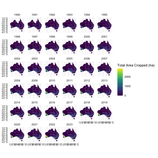
Plot of AAGIS estimated total area cropped by year and region.
Working With AGFD Data
You can download files and pipe directly into the class object that you desire for the Australian Farm Gridded Data (AGFD) data.
Description of the Australian Farm Gridded Data
Directly from the DAFF website:
The Australian Gridded Farm Data are a set of national scale maps containing simulated data on historical broadacre farm business outcomes including farm profitability on an 0.05-degree (approximately 5 km) grid.
These data have been produced by ABARES as part of the ongoing Australian Agricultural Drought Indicator (AADI) project (previously known as the Drought Early Warning System Project) and were derived using ABARES farmpredict model, which in turn is based on ABARES Agricultural and Grazing Industries Survey (AAGIS) data.
These maps provide estimates of farm business profit, revenue, costs and production by location (grid cell) and year for the period 1990-91 to 2022-23. The data do not include actual observed outcomes but rather model predicted outcomes for representative or ‘typical’ broadacre farm businesses at each location considering likely farm characteristics and prevailing weather conditions and commodity prices.
The Australian Gridded Farm Data remain under active development, and as such should be considered experimental.
– Australian Department of Agriculture, Fisheries and Forestry.
Download and read the AGFD files as a list of {stars} objects returning only data for the year 2000.
# A list of {stars} objects for the climate in year 2000
star <- read_agfd_stars(2000)
#> no 'var' specified, using farmno, R_total_hat_ha, C_total_hat_ha, FBP_fci_hat_ha, FBP_fbp_hat_ha, A_wheat_hat_ha, H_wheat_dot_hat, A_barley_hat_ha, H_barley_dot_hat, A_sorghum_hat_ha, H_sorghum_dot_hat, A_oilseeds_hat_ha, H_oilseeds_dot_hat, R_wheat_hat_ha, R_sorghum_hat_ha, R_oilseeds_hat_ha, R_barley_hat_ha, Q_wheat_hat_ha, Q_barley_hat_ha, Q_sorghum_hat_ha, Q_oilseeds_hat_ha, S_wheat_cl_hat_ha, S_sheep_cl_hat_ha, S_sheep_births_hat_ha, S_sheep_deaths_hat_ha, S_beef_cl_hat_ha, S_beef_births_hat_ha, S_beef_deaths_hat_ha, Q_beef_hat_ha, Q_sheep_hat_ha, Q_lamb_hat_ha, R_beef_hat_ha, R_sheep_hat_ha, R_lamb_hat_ha, C_fodder_hat_ha, C_fert_hat_ha, C_fuel_hat_ha, C_chem_hat_ha, A_total_cropped_ha, FBP_pfe_hat_ha, farmland_per_cell
#> other available variables:
#>  lon, lat
#> Will return stars object with 612226 cells.
#> No projection information found in nc file.
#>  Coordinate variable units found to be degrees,
#>  assuming WGS84 Lat/Lon.

head(star[[1]])
#> stars object with 2 dimensions and 6 attributes
#> attribute(s):
#>                         Min.         1st Qu.         Median           Mean
#> farmno          15612.000000 233091.50000000 329567.0000000 324737.7187618
#> R_total_hat_ha      3.105843      7.09662085     19.7569846    169.1918352
#> C_total_hat_ha      1.282748      4.27412711      9.8605795     94.1287971
#> FBP_fci_hat_ha   -134.049904      2.86625943      9.8397018     75.0630380
#> FBP_fbp_hat_ha   -328.818624      3.42896902     12.3912337     63.5968722
#> A_wheat_hat_ha      0.000000      0.04116083      0.1126724      0.1368933
#>                        3rd Qu.           Max.   NA's
#> farmno          418508.5000000 669706.0000000 443899
#> R_total_hat_ha     161.2597086   2459.0029014 443899
#> C_total_hat_ha      92.5196069   1908.2287127 443899
#> FBP_fci_hat_ha      66.9675602   1224.9113170 443899
#> FBP_fbp_hat_ha      59.2320889   1214.8330655 443899
#> A_wheat_hat_ha       0.2099372      0.5107011 565224
#> dimension(s):
#>     from  to         refsys              values x/y
#> lon    1 886 WGS 84 (CRS84) [886] 112,...,156.2 [x]
#> lat    1 691 WGS 84 (CRS84) [691] -44.5,...,-10 [y]
Download and read the AGFD files as a terra::rast object.
# A {terra} `rast` object
terr <- read_agfd_terra(2000)

head(terr[[1]])
#> class       : SpatRaster
#> size        : 6, 886, 41  (nrow, ncol, nlyr)
#> resolution  : 0.05, 0.05  (x, y)
#> extent      : 111.975, 156.275, -10.275, -9.975  (xmin, xmax, ymin, ymax)
#> coord. ref. : lon/lat WGS 84 (CRS84) (OGC:CRS84)
#> source(s)   : memory
#> names       : farmno, R_tot~at_ha, C_tot~at_ha, FBP_f~at_ha, FBP_f~at_ha, A_whe~at_ha, ...
#> min values  :    NaN,         NaN,         NaN,         NaN,         NaN,         NaN, ...
#> max values  :    NaN,         NaN,         NaN,         NaN,         NaN,         NaN, ...
Download and read the AGFD files as a list of {tidync} objects.
# A list of {tidync} objects
tdnc <- read_agfd_tidync(2000)

head(tdnc[[1]])
#> $source
#> # A tibble: 1 × 2
#>   access              source
#>   <dttm>              <chr>
#> 1 2025-12-14 09:31:46 /private/var/folders/vz/txwj1tx51txgw7zv_b5c5_3m0000gn/T/…
#>
#> $axis
#> # A tibble: 84 × 3
#>     axis variable       dimension
#>    <int> <chr>              <int>
#>  1     1 lon                    0
#>  2     2 lat                    1
#>  3     3 farmno                 0
#>  4     4 farmno                 1
#>  5     5 R_total_hat_ha         0
#>  6     6 R_total_hat_ha         1
#>  7     7 C_total_hat_ha         0
#>  8     8 C_total_hat_ha         1
#>  9     9 FBP_fci_hat_ha         0
#> 10    10 FBP_fci_hat_ha         1
#> # ℹ 74 more rows
#>
#> $grid
#> # A tibble: 3 × 4
#>   grid  ndims variables         nvars
#>   <chr> <int> <list>            <int>
#> 1 D0,D1     2 <tibble [41 × 1]>    41
#> 2 D0        1 <tibble [1 × 1]>      1
#> 3 D1        1 <tibble [1 × 1]>      1
#>
#> $dimension
#> # A tibble: 2 × 8
#>      id name  length unlim coord_dim active start count
#>   <int> <chr>  <dbl> <lgl> <lgl>     <lgl>  <int> <int>
#> 1     0 lon      886 FALSE TRUE      TRUE       1   886
#> 2     1 lat      691 FALSE TRUE      TRUE       1   691
#>
#> $variable
#> # A tibble: 43 × 7
#>       id name            type      ndims natts dim_coord active
#>    <int> <chr>           <chr>     <int> <int> <lgl>     <lgl>
#>  1     0 lon             NC_DOUBLE     1     2 TRUE      FALSE
#>  2     1 lat             NC_DOUBLE     1     2 TRUE      FALSE
#>  3     2 farmno          NC_DOUBLE     2     1 FALSE     TRUE
#>  4     3 R_total_hat_ha  NC_DOUBLE     2     1 FALSE     TRUE
#>  5     4 C_total_hat_ha  NC_DOUBLE     2     1 FALSE     TRUE
#>  6     5 FBP_fci_hat_ha  NC_DOUBLE     2     1 FALSE     TRUE
#>  7     6 FBP_fbp_hat_ha  NC_DOUBLE     2     1 FALSE     TRUE
#>  8     7 A_wheat_hat_ha  NC_DOUBLE     2     1 FALSE     TRUE
#>  9     8 H_wheat_dot_hat NC_DOUBLE     2     1 FALSE     TRUE
#> 10     9 A_barley_hat_ha NC_DOUBLE     2     1 FALSE     TRUE
#> # ℹ 33 more rows
#>
#> $attribute
#> # A tibble: 49 × 4
#>       id name       variable       value
#>    <int> <chr>      <chr>          <named list>
#>  1     0 _FillValue lon            <dbl [1]>
#>  2     1 units      lon            <chr [1]>
#>  3     0 _FillValue lat            <dbl [1]>
#>  4     1 units      lat            <chr [1]>
#>  5     0 _FillValue farmno         <dbl [1]>
#>  6     0 _FillValue R_total_hat_ha <dbl [1]>
#>  7     0 _FillValue C_total_hat_ha <dbl [1]>
#>  8     0 _FillValue FBP_fci_hat_ha <dbl [1]>
#>  9     0 _FillValue FBP_fbp_hat_ha <dbl [1]>
#> 10     0 _FillValue A_wheat_hat_ha <dbl [1]>
#> # ℹ 39 more rows
Download and read the AGFD files as a {data.table} object.
# A {data.table} object
dtbl <- read_agfd_dt(2000)

#Check the completeness and other metadata about the data
library(skimr)
skim(dtbl)| Name | dtbl |
| Number of rows | 168327 |
| Number of columns | 44 |
| Key | NULL |
| _______________________ | |
| Column type frequency: | |
| character | 1 |
| numeric | 43 |
| ________________________ | |
| Group variables | None |
Variable type: character
| skim_variable | n_missing | complete_rate | min | max | empty | n_unique | whitespace |
|---|---|---|---|---|---|---|---|
| id | 0 | 1 | 26 | 26 | 0 | 1 | 0 |
Variable type: numeric
| skim_variable | n_missing | complete_rate | mean | sd | p0 | p25 | p50 | p75 | p100 | hist |
|---|---|---|---|---|---|---|---|---|---|---|
| farmno | 0 | 1.00 | 324737.72 | 119413.06 | 15612.00 | 233091.50 | 329567.00 | 418508.50 | 669706.00 | ▂▆▇▆▁ |
| R_total_hat_ha | 0 | 1.00 | 169.19 | 303.84 | 3.11 | 7.10 | 19.76 | 161.26 | 2459.00 | ▇▁▁▁▁ |
| C_total_hat_ha | 0 | 1.00 | 94.13 | 169.85 | 1.28 | 4.27 | 9.86 | 92.52 | 1908.23 | ▇▁▁▁▁ |
| FBP_fci_hat_ha | 0 | 1.00 | 75.06 | 139.61 | -134.05 | 2.87 | 9.84 | 66.97 | 1224.91 | ▇▁▁▁▁ |
| FBP_fbp_hat_ha | 0 | 1.00 | 63.60 | 113.65 | -328.82 | 3.43 | 12.39 | 59.23 | 1214.83 | ▁▇▁▁▁ |
| A_wheat_hat_ha | 121325 | 0.28 | 0.14 | 0.12 | 0.00 | 0.04 | 0.11 | 0.21 | 0.51 | ▇▅▂▂▁ |
| H_wheat_dot_hat | 129784 | 0.23 | 2.46 | 0.92 | 0.42 | 1.69 | 2.44 | 3.12 | 5.43 | ▃▇▇▃▁ |
| A_barley_hat_ha | 121325 | 0.28 | 0.06 | 0.06 | 0.00 | 0.00 | 0.05 | 0.09 | 0.29 | ▇▃▂▁▁ |
| H_barley_dot_hat | 134701 | 0.20 | 2.41 | 0.75 | 0.03 | 1.91 | 2.43 | 2.92 | 4.98 | ▁▅▇▃▁ |
| A_sorghum_hat_ha | 152991 | 0.09 | 0.02 | 0.04 | 0.00 | 0.00 | 0.00 | 0.00 | 0.25 | ▇▁▁▁▁ |
| H_sorghum_dot_hat | 165558 | 0.02 | 3.47 | 0.99 | 1.39 | 2.67 | 3.32 | 4.24 | 6.51 | ▃▇▅▃▁ |
| A_oilseeds_hat_ha | 121325 | 0.28 | 0.05 | 0.05 | 0.00 | 0.00 | 0.02 | 0.09 | 0.30 | ▇▃▂▁▁ |
| H_oilseeds_dot_hat | 144457 | 0.14 | 1.64 | 0.47 | 0.32 | 1.34 | 1.66 | 1.98 | 3.02 | ▂▅▇▅▁ |
| R_wheat_hat_ha | 121325 | 0.28 | 122.86 | 124.40 | 0.00 | 19.52 | 79.59 | 201.29 | 894.12 | ▇▃▁▁▁ |
| R_sorghum_hat_ha | 152991 | 0.09 | 13.24 | 35.84 | 0.00 | 0.04 | 0.23 | 1.66 | 375.66 | ▇▁▁▁▁ |
| R_oilseeds_hat_ha | 121325 | 0.28 | 51.46 | 66.99 | 0.00 | 0.00 | 9.76 | 95.01 | 619.06 | ▇▁▁▁▁ |
| R_barley_hat_ha | 121325 | 0.28 | 44.12 | 56.62 | 0.00 | 0.29 | 21.32 | 63.49 | 309.55 | ▇▂▁▁▁ |
| Q_wheat_hat_ha | 121325 | 0.28 | 0.33 | 0.34 | 0.00 | 0.05 | 0.21 | 0.53 | 2.26 | ▇▃▁▁▁ |
| Q_barley_hat_ha | 121325 | 0.28 | 0.12 | 0.16 | 0.00 | 0.00 | 0.06 | 0.18 | 0.89 | ▇▂▁▁▁ |
| Q_sorghum_hat_ha | 152991 | 0.09 | 0.05 | 0.13 | 0.00 | 0.00 | 0.00 | 0.00 | 1.50 | ▇▁▁▁▁ |
| Q_oilseeds_hat_ha | 121325 | 0.28 | 0.08 | 0.10 | 0.00 | 0.00 | 0.02 | 0.15 | 0.76 | ▇▂▁▁▁ |
| S_wheat_cl_hat_ha | 121325 | 0.28 | 0.05 | 0.05 | 0.00 | 0.01 | 0.03 | 0.07 | 0.43 | ▇▂▁▁▁ |
| S_sheep_cl_hat_ha | 0 | 1.00 | 0.20 | 0.52 | 0.00 | 0.00 | 0.00 | 0.09 | 5.07 | ▇▁▁▁▁ |
| S_sheep_births_hat_ha | 0 | 1.00 | 0.14 | 0.36 | 0.00 | 0.00 | 0.00 | 0.06 | 3.90 | ▇▁▁▁▁ |
| S_sheep_deaths_hat_ha | 0 | 1.00 | 0.01 | 0.03 | 0.00 | 0.00 | 0.00 | 0.01 | 0.34 | ▇▁▁▁▁ |
| S_beef_cl_hat_ha | 0 | 1.00 | 0.07 | 0.14 | 0.00 | 0.01 | 0.02 | 0.06 | 1.87 | ▇▁▁▁▁ |
| S_beef_births_hat_ha | 0 | 1.00 | 0.03 | 0.06 | 0.00 | 0.00 | 0.01 | 0.02 | 0.75 | ▇▁▁▁▁ |
| S_beef_deaths_hat_ha | 0 | 1.00 | 0.00 | 0.00 | 0.00 | 0.00 | 0.00 | 0.00 | 0.04 | ▇▁▁▁▁ |
| Q_beef_hat_ha | 0 | 1.00 | 0.02 | 0.05 | 0.00 | 0.00 | 0.01 | 0.02 | 0.70 | ▇▁▁▁▁ |
| Q_sheep_hat_ha | 0 | 1.00 | 0.08 | 0.20 | 0.00 | 0.00 | 0.00 | 0.03 | 2.47 | ▇▁▁▁▁ |
| Q_lamb_hat_ha | 0 | 1.00 | 0.09 | 0.25 | 0.00 | 0.00 | 0.00 | 0.03 | 3.27 | ▇▁▁▁▁ |
| R_beef_hat_ha | 0 | 1.00 | 50.65 | 129.53 | 0.00 | 3.99 | 12.45 | 31.13 | 1785.92 | ▇▁▁▁▁ |
| R_sheep_hat_ha | 0 | 1.00 | 14.20 | 35.77 | 0.00 | 0.03 | 0.26 | 5.82 | 442.53 | ▇▁▁▁▁ |
| R_lamb_hat_ha | 0 | 1.00 | 18.30 | 50.75 | 0.00 | 0.00 | 0.15 | 5.33 | 645.74 | ▇▁▁▁▁ |
| C_fodder_hat_ha | 0 | 1.00 | 4.51 | 10.33 | 0.06 | 0.22 | 0.74 | 3.73 | 197.98 | ▇▁▁▁▁ |
| C_fert_hat_ha | 0 | 1.00 | 16.65 | 35.99 | 0.00 | 0.01 | 0.05 | 8.92 | 367.57 | ▇▁▁▁▁ |
| C_fuel_hat_ha | 0 | 1.00 | 5.64 | 9.81 | 0.12 | 0.35 | 0.66 | 6.04 | 110.46 | ▇▁▁▁▁ |
| C_chem_hat_ha | 0 | 1.00 | 9.27 | 21.28 | 0.00 | 0.00 | 0.02 | 4.71 | 195.40 | ▇▁▁▁▁ |
| A_total_cropped_ha | 0 | 1.00 | 0.07 | 0.16 | 0.00 | 0.00 | 0.00 | 0.03 | 0.82 | ▇▁▁▁▁ |
| FBP_pfe_hat_ha | 0 | 1.00 | 70.04 | 123.69 | -291.84 | 3.65 | 12.94 | 67.12 | 1314.10 | ▇▃▁▁▁ |
| farmland_per_cell | 0 | 1.00 | 2060.59 | 616.84 | 61.72 | 1752.29 | 2188.27 | 2463.95 | 3024.09 | ▁▁▃▇▅ |
| lon | 0 | 1.00 | 136.82 | 10.76 | 113.15 | 130.55 | 139.95 | 145.05 | 153.60 | ▃▂▃▇▅ |
| lat | 0 | 1.00 | -26.21 | 5.97 | -43.45 | -30.90 | -26.45 | -21.65 | -10.75 | ▁▆▇▆▂ |
Working With the Soil Thickness Map
You can download the soil depth map and import it as a {stars} or terra::rast() object.
ts_t <- read_topsoil_thickness_terra()
ts_s <- read_topsoil_thickness_stars()
For your convenience, {read.abares} re-exports terra::plot(),
so you can just use plot() with the {terra} objects in
{read.abares}, by default {stars} already handles plot
gracefully.
plot(ts_t)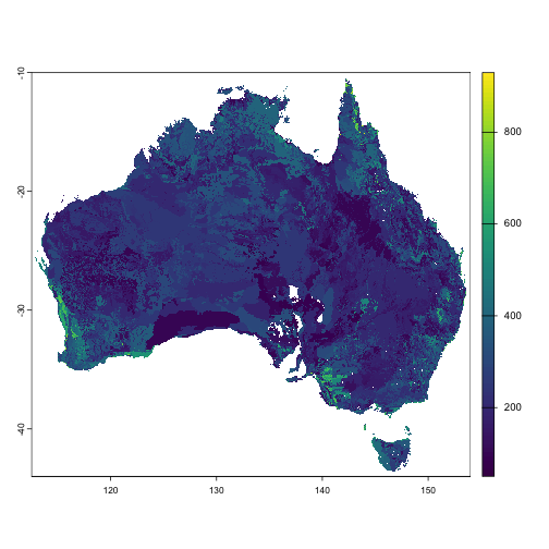
Soil Thickness for Australian areas of intensive agriculture of Layer 1 (A Horizon - top-soil) (derived from soil mapping)
Soil Thickness Metadata
The topsoil thickness data object will contain the associated metadata no matter which R package you choose, {terra} or {stars}.
print_topsoil_thickness_metadata()
#>
#> ── Topsoil Thickness for Australian areas of intensive agriculture of Layer 1 (A
#>
#> ── Dataset ANZLIC ID ANZCW1202000149 ──
#>
#> Custodian CSIRO, Land & Water
#>
#> Jurisdiction Australia
#>
#> Description Abstract Surface of predicted Thickness of soil layer 1 (A Horizon
#> - top-soil) surface for the intensive agricultural areas of Australia.  Data
#> modelled from area based observations made by soil agencies both State and
#> CSIRO and presented as .0.01 degree grid cells.
#>
#> Topsoils (A horizons) are defined as the surface soil layers in which organic
#> matter accumulates, and may include dominantly organic surface layers (O and P
#> horizons).
#>
#> The depth of topsoil is important because, with their higher organic matter
#> contents, topsoils (A horizon) generally have more suitable properties for
#> agriculture, including higher permeability and higher levels of soil nutrients.
#>
#> Estimates of soil depths are needed to calculate the amount of any soil
#> constituent in either volume or mass terms (bulk density is also needed) - for
#> example, the volume of water stored in the rooting zone potentially available
#> for plant use, to assess total stores of soil carbon for Greenhouse inventory
#> or to assess total stores of nutrients.
#>
#> The pattern of soil depth is strongly related to topography - the shape and
#> slope of the land.  Deeper soils are typically found in the river valleys where
#> soils accumulate on floodplains and at the footslopes of ranges (zones of
#> deposition), while soils on hillslopes (zones of erosion) tend to be shallow.
#> Map of thickness of topsoil was derived from soil map data and interpreted
#> tables of soil properties for specific soil groups.
#>
#> The quality of data on soil depth in existing soil profile datasets is
#> questionable and as the thickness of soil horizons varies locally with
#> topography, values for map units are general averages.
#>
#> The final ASRIS polygon attributed surfaces are a mosaic of all of the data
#> obtained from various state and federal agencies. The surfaces have been
#> constructed with the best available soil survey information available at the
#> time. The surfaces also rely on a number of assumptions. One being that an area
#> weighted mean is a good estimate of the soil attributes for that polygon or
#> map-unit. Another assumption made is that the look-up tables provided by
#> McKenzie et al. (2000), state and territories accurately depict the soil
#> attribute values for each soil type.
#>
#> The accuracy of the maps is most dependent on the scale of the original polygon
#> data sets and the level of soil survey that has taken place in each state.  The
#> scale of the various soil maps used in deriving this map is available by
#> accessing the data-source grid, the scale is used as an assessment of the
#> likely accuracy of the modelling.  The Atlas of Australian Soils is considered
#> to be the least accurate dataset and has therefore only been used where there
#> is no state based data.  Of the state datasets Western Australian sub-systems,
#> South Australian land systems and NSW soil landscapes and reconnaissance
#> mapping would be the most reliable based on scale. NSW soil landscapes and
#> reconnaissance mapping use only one dominant soil type per polygon in the
#> estimation of attributes.  South Australia and Western Australia use several
#> soil types per polygon or map-unit.
#>
#> The digital map data is provided in geographical coordinates based on the World
#> Geodetic System 1984 (WGS84) datum. This raster data set has a grid resolution
#> of 0.001 degrees (approximately equivalent to 1.1 km).
#>
#> The data set is a product of the National Land and Water Resources Audit
#> (NLWRA) as a base dataset.
#>
#> Search Word(s) AGRICULTURE SOIL Physics Models
#>
#> Geographic Extent Name(s) GEN Category
#>
#> GEN Custodial Jurisdiction
#>
#> GEN Name
#>
#> Geographic Bounding Box North Bounding Latitude -10.707149 South Bounding
#> Latitude -43.516831 East Bounding Longitude 113.19673 West Bounding Longitude
#> 153.990779
#>
#> Geographic Extent Polygon(s) 115.0 -33.5,115.7 -33.3,115.7 -31.7,113.2
#> -26.2,113.5 -25.4,114.1 -26.4,114.3 -26.0,113.4 -24.3,114.1 -21.8,122.3
#> -18.2,122.2 -17.2,126.7 -13.6,129.1 -14.9,130.6 -12.3,132.6 -12.1,132.5
#> -11.6,131.9 -11.3,132.0 -11.1,137.0 -12.2,135.4 -14.7,140.0 -17.7,140.8
#> -17.4,141.7 -15.1,141.4 -13.7,142.2 -10.9,142.7 -10.7,143.9 -14.5,144.6
#> -14.1,145.3 -14.9,146.3 -18.8,148.9 -20.5,150.9 -22.6,153.2 -25.9,153.7
#> -28.8,153.0 -31.3,150.8 -34.8,150.0 -37.5,147.8 -37.9,146.3 -39.0,144.7
#> -38.4,143.5 -38.8,141.3 -38.4,139.7 -37.3,139.7 -36.9,139.9 -36.7,138.9
#> -35.5,138.1 -35.7,138.6 -34.7,138.1 -34.2,137.8 -35.1,136.9 -35.3,137.0
#> -34.9,137.5 -34.9,137.4 -34.0,137.9 -33.5,137.8 -32.6,137.3 -33.6,135.9
#> -34.7,136.1 -34.8,136.0 -35.0,135.1 -34.6,135.2 -34.5,135.4 -34.5,134.7
#> -33.3,134.0 -32.9,133.7 -32.1,133.3 -32.2,132.2 -32.0,131.3 -31.5,127.3
#> -32.3,126.0 -32.3,123.6 -33.9,123.2 -34.0,122.1 -34.0,121.9 -33.8,119.9
#> -34.0,119.6 -34.4,118.0 -35.1,116.0 -34.8,115.0 -34.3,115.0 -33.5
#>
#> 147.8 -42.9,147.9 -42.6,148.2 -42.1,148.3 -42.3,148.3 -41.3,148.3 -41.0,148.0
#> -40.7,147.4 -41.0,146.7 -41.1,146.6 -41.2,146.5 -41.1,146.4 -41.2,145.3
#> -40.8,145.3 -40.7,145.2 -40.8,145.2 -40.8,145.2 -40.8,145.0 -40.8,144.7
#> -40.7,144.7 -41.2,145.2 -42.2,145.4 -42.2,145.5 -42.4,145.5 -42.5,145.2
#> -42.3,145.5 -43.0,146.0 -43.3,146.0 -43.6,146.9 -43.6,146.9 -43.5,147.1
#> -43.3,147.0 -43.1,147.2 -43.3,147.3 -42.8,147.4 -42.9,147.6 -42.8,147.5
#> -42.8,147.8 -42.9,147.9 -43.0,147.7 -43.0,147.8 -43.2,147.9 -43.2,147.9
#> -43.2,148.0 -43.2,148.0 -43.1,148.0 -42.9,147.8 -42.9
#>
#> 136.7 -13.8,136.7 -13.7,136.6 -13.7,136.6 -13.8,136.4 -13.8,136.4 -14.1,136.3
#> -14.2,136.9 -14.3,137.0 -14.2,136.9 -14.2,136.7 -14.1,136.9 -13.8,136.7
#> -13.8,136.7 -13.8
#>
#> 139.5 -16.6,139.7 -16.5,139.4 -16.5,139.2 -16.7,139.3 -16.7,139.5 -16.6
#>
#> 153.0 -25.2,153.0 -25.7,153.1 -25.8,153.4 -25.0,153.2 -24.7,153.2 -25.0,153.0
#> -25.2
#>
#> 137.5 -36.1,137.7 -35.9,138.1 -35.9,137.9 -35.7,137.6 -35.7,137.6 -35.6,136.6
#> -35.8,136.7 -36.1,137.2 -36.0,137.5 -36.1
#>
#> 143.9 -39.7,144.0 -39.6,144.1 -39.8,143.9 -40.2,143.9 -40.0,143.9 -39.7
#>
#> 148.0 -39.7,147.7 -39.9,147.9 -39.9,148.0 -40.1,148.1 -40.3,148.3 -40.2,148.3
#> -40.0,148.0 -39.7
#>
#> 148.1 -40.4,148.0 -40.4,148.4 -40.3,148.4 -40.5,148.1 -40.4
#>
#> 130.4 -11.3,130.4 -11.2,130.6 -11.3,130.7 -11.4,130.9 -11.3,131.0 -11.4,131.1
#> -11.3,131.2 -11.4,131.3 -11.2,131.5 -11.4,131.5 -11.5,131.0 -11.9,130.8
#> -11.8,130.6 -11.7,130.0 -11.8,130.1 -11.7,130.3 -11.7,130.1 -11.5,130.4 -11.3
#>
#> Data Currency Beginning date 1999-09-01
#>
#> Ending date 2001-03-31
#>
#> Dataset Status Progress COMPLETE
#>
#> Maintenance and Update Frequency NOT PLANNED
#>
#> Access Stored Data Format DIGITAL - ESRI Arc/Info integer GRID
#>
#> Available Format Type DIGITAL - ESRI Arc/Info integer GRID
#>
#> Access Constraint Subject to the terms & condition of the data access &
#> management agreement between the National Land & Water Audit and ANZLIC parties
#>
#> Data Quality Lineage The soil attribute surface was created using the following
#> datasets 1. The digital polygon coverage of the Soil-Landforms of the Murray
#> Darling Basis (MDBSIS)(Bui et al. 1998), classified as principal profile forms
#> (PPF's) (Northcote 1979). 2. The digital Atlas of Australian Soils (Northcote
#> et al.1960-1968)(Leahy, 1993). 3. Western Australia land systems coverage
#> (Agriculture WA). 4. Western Australia sub-systems coverage (Agriculture WA).
#> 5. Ord river catchment soils coverage (Agriculture WA). 6. Victoria soils
#> coverage (Victorian Department of Natural Resources and Environment - NRE). 7.
#> NSW Soil Landscapes and reconnaissance soil landscape mapping (NSW Department
#> of Land and Water Conservation - DLWC). 8. New South Wales Land systems west
#> (NSW Department of Land and Water Conservation - DLWC). 9. South Australia soil
#> land-systems (Primary Industries and Resources South Australia - PIRSA). 10.
#> Northern Territory soils coverage (Northern Territory Department of Lands,
#> Planning and Environment). 11. A mosaic of Queensland soils coverages
#> (Queensland Department of Natural Resources - QDNR). 12. A look-up table
#> linking PPF values from the Atlas of Australian Soils with interpreted soil
#> attributes (McKenzie et al. 2000). 13. Look_up tables provided by WA
#> Agriculture linking WA soil groups with interpreted soil attributes. 14.
#> Look_up tables provided by PIRSA linking SA soil groups with interpreted soil
#> attributes.
#>
#> The continuous raster surface representing Thickness of soil layer 1 was
#> created by combining national and state level digitised land systems maps and
#> soil surveys linked to look-up tables listing soil type and corresponding
#> attribute values.
#>
#> Because thickness is used sparingly in the Factual Key, estimations of
#> thickness in the look-up tables were made using empirical correlations for
#> particular soil types.
#>
#> To estimate a soil attribute where more than one soil type was given for a
#> polygon or map-unit, the soil attribute values related to each soil type in the
#> look-up table were weighted according to the area occupied by that soil type
#> within the polygon or map-unit. The final soil attribute values are an area
#> weighted average for a polygon or map-unit.  The polygon data was then
#> converted to a continuous raster surface using the soil attribute values
#> calculated for each polygon.
#>
#> The ASRIS soil attribute surfaces created using polygon attribution relied on a
#> number of data sets from various state agencies.  Each polygon data set was
#> turned into a continuous surface grid based on the calculated soil attribute
#> value for that polygon.  The grids where then merged on the basis that, where
#> available, state data replaced the Atlas of Australian Soils and MDBSIS.
#> MDBSIS derived soil attribute values were restricted to areas where MDBSIS was
#> deemed to be more accurate that the Atlas of Australian Soils (see Carlile et
#> al (2001a).
#>
#> In cases where a soil type was missing from the look-up table or layer 2 did
#> not exist for that soil type, the percent area of the soils remaining were
#> adjusted prior to calculating the final soil attribute value. The method used
#> to attribute polygons was dependent on the data supplied by individual State
#> agencies.
#>
#> The modelled grid was resampled from 0.0025 degree cells to 0.01 degree cells
#> using bilinear interpolation
#>
#> Positional Accuracy The predictive surface is a 0.01 X 0.01 degree grid and has
#> a locational accurate of about 1m.
#>
#> The positional accuracy of the defining polygons have variable positional
#> accuracy most locations are expected to be within 100m of the recorded
#> location.  The vertical accuracy is not relevant. The positional assessment has
#> been made by considering the tools used to generate the locational information
#> and contacting the data providers.
#>
#> The other parameters used in the production of the led surface have a range of
#> positional accuracy ranging from + - 50 m to + - kilometres.  This contribute
#> to the loss of attribute accuracy in the surface.
#>
#> Attribute Accuracy Input attribute accuracy for the areas is highly variable.
#> The predictive has a variable and much lower attribute accuracy due to the
#> irregular distribution and the limited positional accuracy of the parameters
#> used for modelling.
#>
#> There are several sources of error in estimating soil depth and thickness of
#> horizons for the look-up tables.  Because thickness is used sparingly in the
#> Factual Key, estimations of thickness in the look-up tables were made using
#> empirical correlations for particular soil types.  The quality of data on soil
#> depth in existing soil profile datasets is questionable, in soil mapping,
#> thickness of soil horizons varies locally with topography, so values for map
#> units are general averages.  The definition of the depth of soil or regolith is
#> imprecise and it can be difficult to determine the lower limit of soil.
#>
#> The assumption made that an area weighted mean of soil attribute values based
#> on soil type is a good estimation of a soil property is debatable, in that it
#> does not supply the soil attribute value at any given location. Rather it is
#> designed to show national and regional patterns in soil properties. The use of
#> the surfaces at farm or catchment scale modelling may prove inaccurate. Also
#> the use of look-up tables to attribute soil types is only as accurate as the
#> number of observations used to estimate a attribute value for a soil type. Some
#> soil types in the look-up tables may have few observations, yet the average
#> attribute value is still taken as the attribute value for that soil type.
#> Different states are using different taxonomic schemes making a national soil
#> database difficult. Another downfall of the area weighted approach is that some
#> soil types may not be listed in look-up tables. If a soil type is a dominant
#> one within a polygon or map-unit, but is not listed within the look-up table or
#> is not attributed within the look-up table then the final soil attribute value
#> for that polygon will be biased towards the minor soil types that do exist.
#> This may also happen when a large area is occupied by a soil type which has no
#> B horizon. In this case the final soil attribute value will be area weighted on
#> the soils with a B horizon, ignoring a major soil type within that polygon or
#> map-unit. The layer 2 surfaces have large areas of no-data because all soils
#> listed for a particular map-unit or polygon had no B horizon.
#>
#> Logical Consistency Surface is fully logically consistent as only one parameter
#> is shown, as predicted average Soil Thickness within each grid cell
#>
#> Completeness Surface is nearly complete.  There are some areas (about %1
#> missing) for which insufficient parameters were known to provide a useful
#> prediction and thus attributes are absent in these areas.
#>
#> Contact Information Contact Organisation (s) CSIRO, Land & Water
#>
#> Contact Position Project Leader
#>
#> Mail Address ACLEP, GPO 1666
#>
#> Locality Canberra
#>
#> State ACT
#>
#> Country AUSTRALIA
#>
#> Postcode 2601
#>
#> Telephone 02 6246 5922
#>
#> Facsimile 02 6246 5965
#>
#> Electronic Mail Address neil.mckenzie@cbr.clw.csiro.au
#>
#> Metadata Date Metadata Date 2001-07-01
#>
#> Additional Metadata Additional Metadata
#>
#> Entity and Attributes Entity Name Soil Thickness Layer 1 (derived from mapping)
#>
#> Entity description Estimated Soil Thickness (mm) of Layer 1 on a cell by cell
#> basis
#>
#> Feature attribute name VALUE
#>
#> Feature attribute definition Predicted average Thickness (mm) of soil layer 1
#> in the 0.01 X 0.01 degree quadrat
#>
#> Data Type Spatial representation type RASTER
#>
#> Projection Map projection GEOGRAPHIC
#>
#> Datum WGS84
#>
#> Map units DECIMAL DEGREES
#>
#> Scale Scale/ resolution 1:1 000 000
#>
#> Usage Purpose Estimates of soil depths are needed to calculate the amount of
#> any soil constituent in either volume or mass terms (bulk density is also
#> needed) - for example, the volume of water stored in the rooting zone
#> potentially available for plant use, to assess total stores of soil carbon for
#> Greenhouse inventory or to assess total stores of nutrients.
#>
#> Provide indications of probable Thickness soil layer 1 in agricultural areas
#> where soil thickness testing has not been carried out
#>
#> Use Use Limitation This dataset is bound by the requirements set down by the
#> National Land & Water Resources Audit